plot.variable generates a
data.frame containing the marginal variable dependence or the
partial variable dependence. The gg_variable function creates a
data.frame of containing the full set of covariate data (predictor
variables) and the predicted response for each observation. Marginal
dependence figures are created using the plot.gg_variable
function.
Optional arguments time point (or vector of points) of interest
(for survival forests only) time_labels If more than one time is
specified, a vector of time labels for differentiating the time points
(for survival forests only) oob indicate if predicted results
should include oob or full data set.
Arguments
- object
a
rfsrcobject- ...
optional arguments
Details
The marginal variable dependence is determined by comparing relation between the predicted response from the randomForest and a covariate of interest.
The gg_variable function operates on a
rfsrc object, or the output from the
plot.variable function.
Examples
## ------------------------------------------------------------
## classification
## ------------------------------------------------------------
## -------- iris data
## iris
rfsrc_iris <- rfsrc(Species ~ ., data = iris)
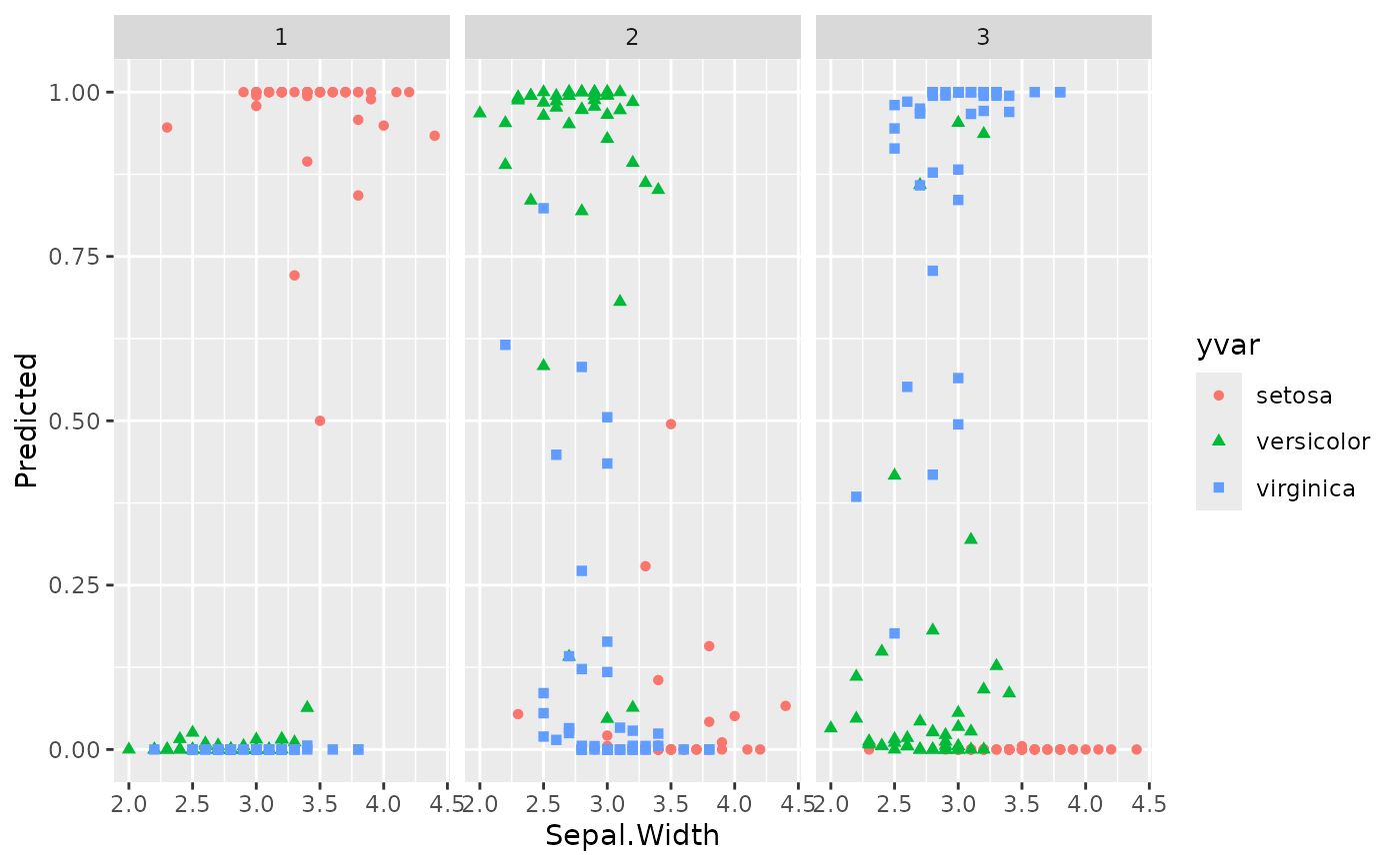
gg_dta <- gg_variable(rfsrc_iris)
plot(gg_dta, xvar = "Sepal.Width")
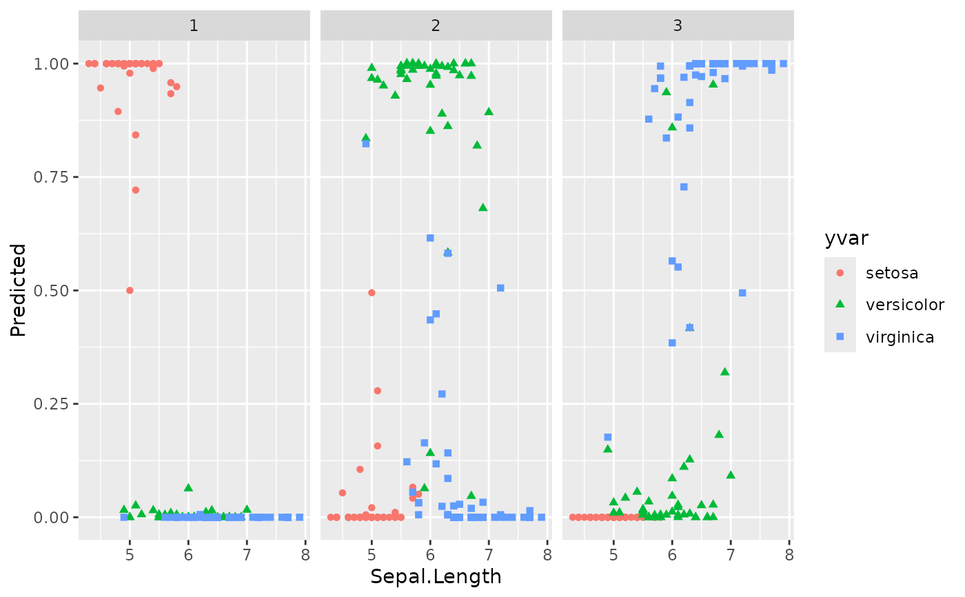
 plot(gg_dta, xvar = "Sepal.Length")
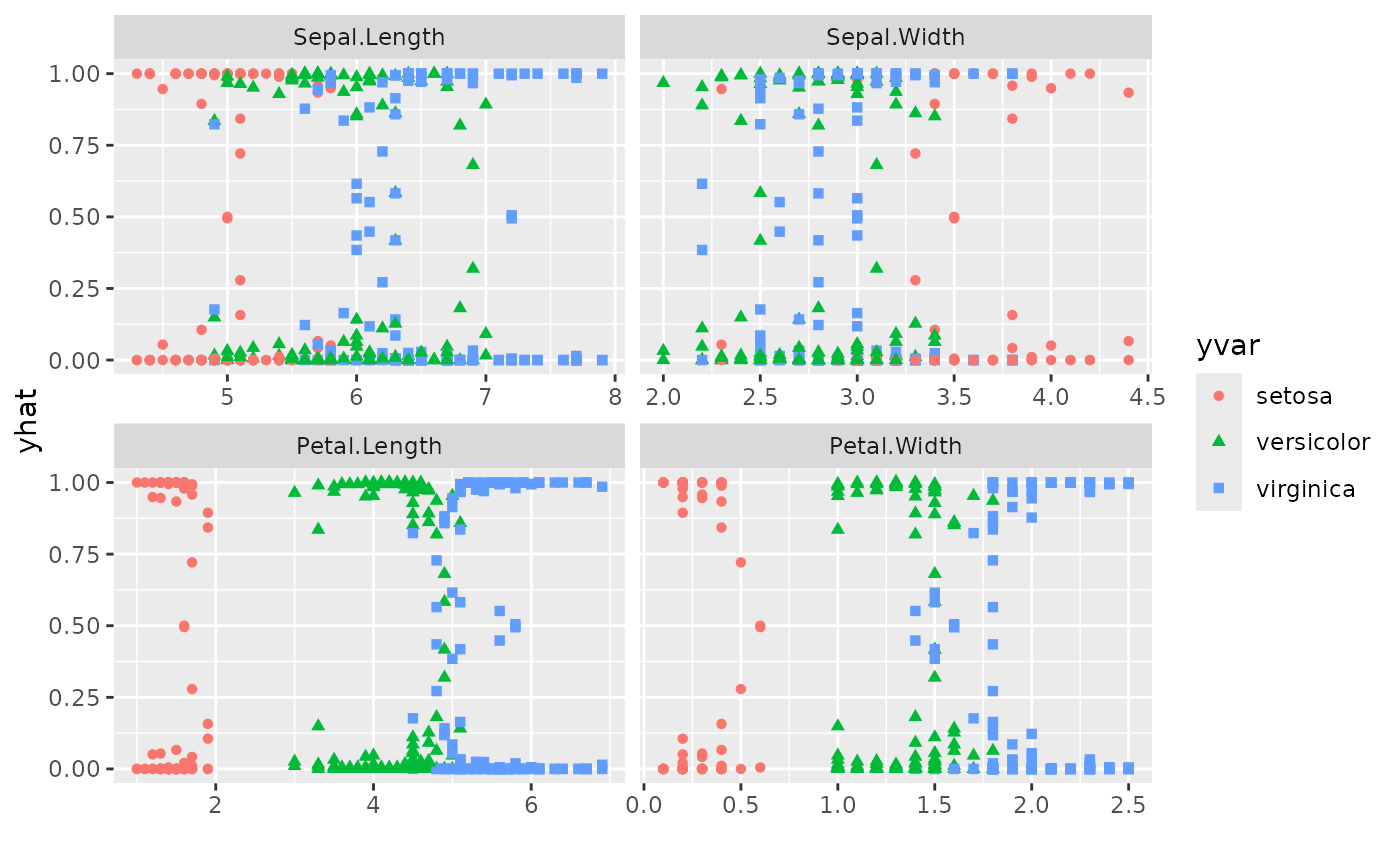
 plot(gg_dta,
xvar = rfsrc_iris$xvar.names,
panel = TRUE
) # , se=FALSE)
plot(gg_dta,
xvar = rfsrc_iris$xvar.names,
panel = TRUE
) # , se=FALSE)
 ## ------------------------------------------------------------
## regression
## ------------------------------------------------------------
## -------- air quality data
rfsrc_airq <- rfsrc(Ozone ~ ., data = airquality)
gg_dta <- gg_variable(rfsrc_airq)
# an ordinal variable
gg_dta[, "Month"] <- factor(gg_dta[, "Month"])
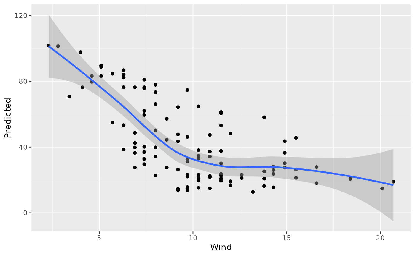
plot(gg_dta, xvar = "Wind")
#> `geom_smooth()` using method = 'loess' and formula = 'y ~ x'
## ------------------------------------------------------------
## regression
## ------------------------------------------------------------
## -------- air quality data
rfsrc_airq <- rfsrc(Ozone ~ ., data = airquality)
gg_dta <- gg_variable(rfsrc_airq)
# an ordinal variable
gg_dta[, "Month"] <- factor(gg_dta[, "Month"])
plot(gg_dta, xvar = "Wind")
#> `geom_smooth()` using method = 'loess' and formula = 'y ~ x'
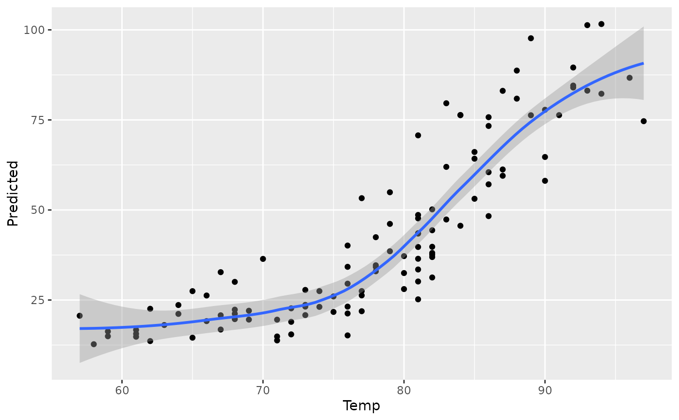
 plot(gg_dta, xvar = "Temp")
#> `geom_smooth()` using method = 'loess' and formula = 'y ~ x'
plot(gg_dta, xvar = "Temp")
#> `geom_smooth()` using method = 'loess' and formula = 'y ~ x'
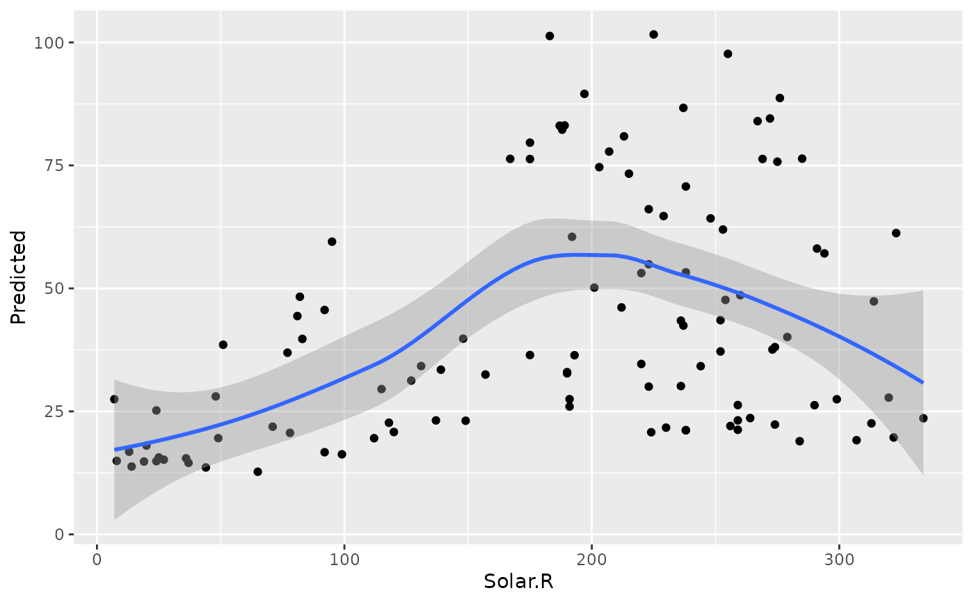
 plot(gg_dta, xvar = "Solar.R")
#> `geom_smooth()` using method = 'loess' and formula = 'y ~ x'
plot(gg_dta, xvar = "Solar.R")
#> `geom_smooth()` using method = 'loess' and formula = 'y ~ x'
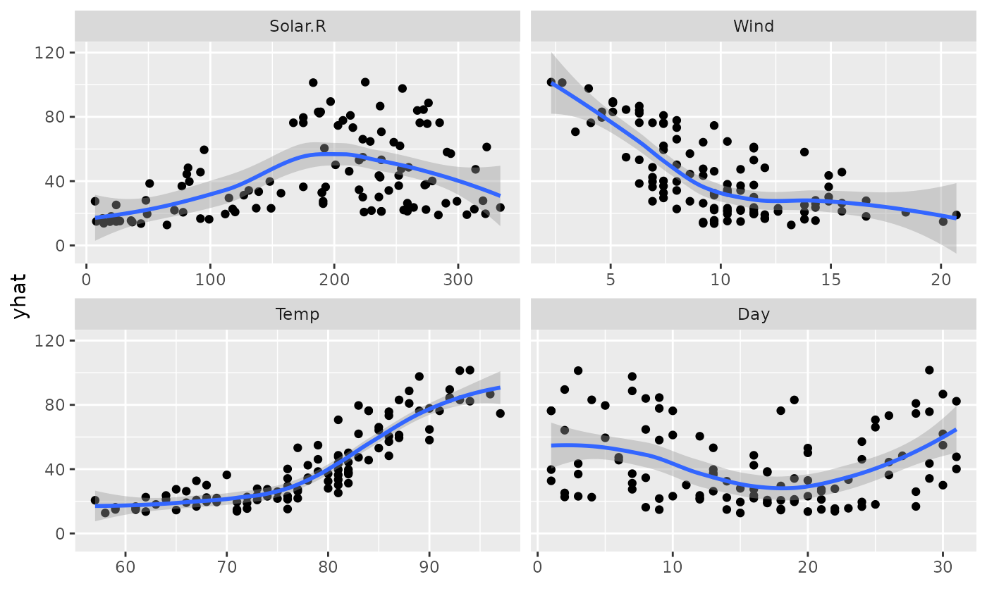
 plot(gg_dta, xvar = c("Solar.R", "Wind", "Temp", "Day"), panel = TRUE)
#> `geom_smooth()` using method = 'loess' and formula = 'y ~ x'
plot(gg_dta, xvar = c("Solar.R", "Wind", "Temp", "Day"), panel = TRUE)
#> `geom_smooth()` using method = 'loess' and formula = 'y ~ x'
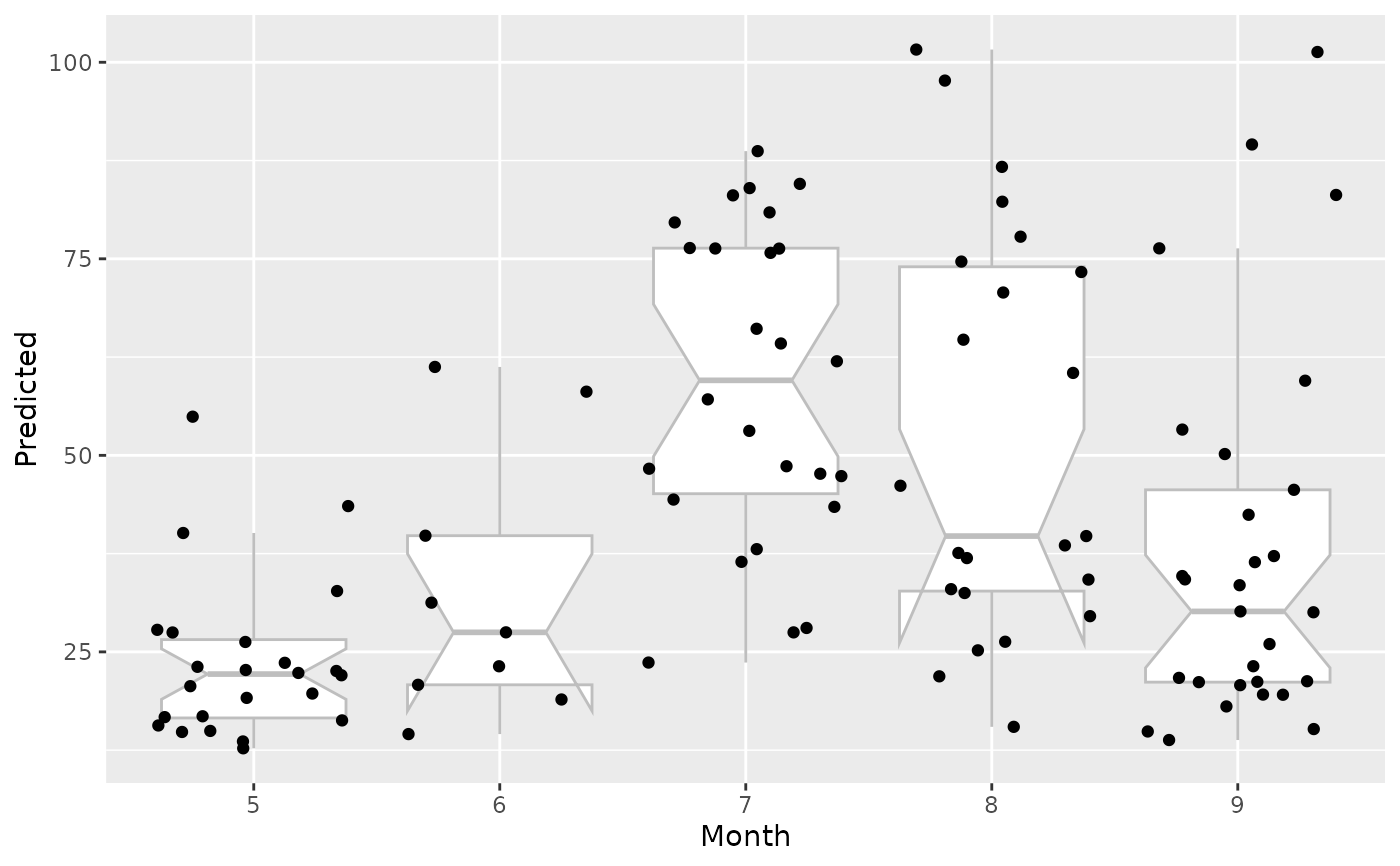
 plot(gg_dta, xvar = "Month", notch = TRUE)
#> Warning: Ignoring unknown parameters: `notch`
#> Notch went outside hinges
#> ℹ Do you want `notch = FALSE`?
#> Notch went outside hinges
#> ℹ Do you want `notch = FALSE`?
plot(gg_dta, xvar = "Month", notch = TRUE)
#> Warning: Ignoring unknown parameters: `notch`
#> Notch went outside hinges
#> ℹ Do you want `notch = FALSE`?
#> Notch went outside hinges
#> ℹ Do you want `notch = FALSE`?
 ## -------- motor trend cars data
rfsrc_mtcars <- rfsrc(mpg ~ ., data = mtcars)
gg_dta <- gg_variable(rfsrc_mtcars)
# mtcars$cyl is an ordinal variable
gg_dta$cyl <- factor(gg_dta$cyl)
gg_dta$am <- factor(gg_dta$am)
gg_dta$vs <- factor(gg_dta$vs)
gg_dta$gear <- factor(gg_dta$gear)
gg_dta$carb <- factor(gg_dta$carb)
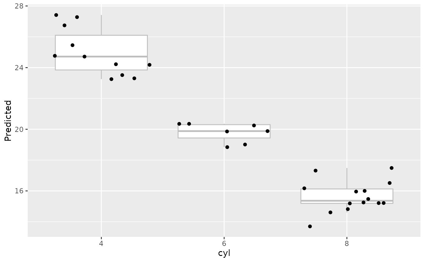
plot(gg_dta, xvar = "cyl")
## -------- motor trend cars data
rfsrc_mtcars <- rfsrc(mpg ~ ., data = mtcars)
gg_dta <- gg_variable(rfsrc_mtcars)
# mtcars$cyl is an ordinal variable
gg_dta$cyl <- factor(gg_dta$cyl)
gg_dta$am <- factor(gg_dta$am)
gg_dta$vs <- factor(gg_dta$vs)
gg_dta$gear <- factor(gg_dta$gear)
gg_dta$carb <- factor(gg_dta$carb)
plot(gg_dta, xvar = "cyl")
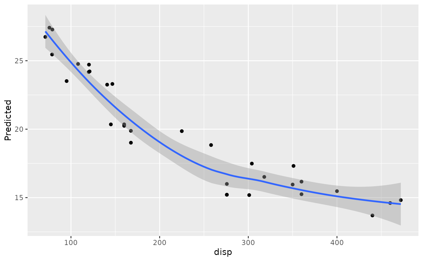
 # Others are continuous
plot(gg_dta, xvar = "disp")
#> `geom_smooth()` using method = 'loess' and formula = 'y ~ x'
# Others are continuous
plot(gg_dta, xvar = "disp")
#> `geom_smooth()` using method = 'loess' and formula = 'y ~ x'
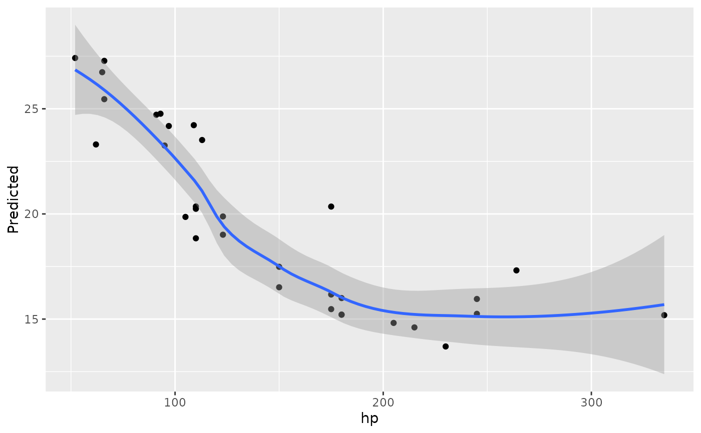
 plot(gg_dta, xvar = "hp")
#> `geom_smooth()` using method = 'loess' and formula = 'y ~ x'
plot(gg_dta, xvar = "hp")
#> `geom_smooth()` using method = 'loess' and formula = 'y ~ x'
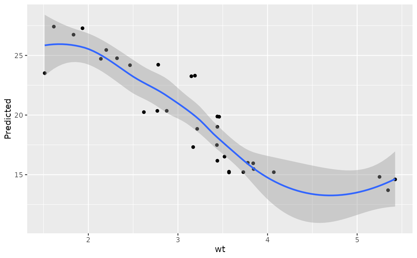
 plot(gg_dta, xvar = "wt")
#> `geom_smooth()` using method = 'loess' and formula = 'y ~ x'
plot(gg_dta, xvar = "wt")
#> `geom_smooth()` using method = 'loess' and formula = 'y ~ x'
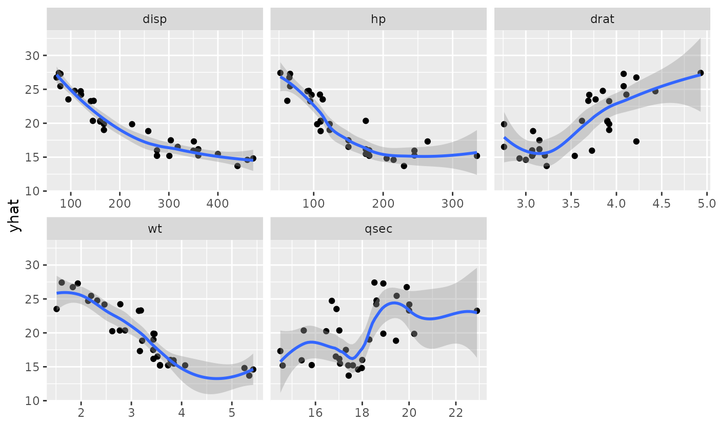
 # panels
plot(gg_dta, xvar = c("disp", "hp", "drat", "wt", "qsec"), panel = TRUE)
#> `geom_smooth()` using method = 'loess' and formula = 'y ~ x'
# panels
plot(gg_dta, xvar = c("disp", "hp", "drat", "wt", "qsec"), panel = TRUE)
#> `geom_smooth()` using method = 'loess' and formula = 'y ~ x'
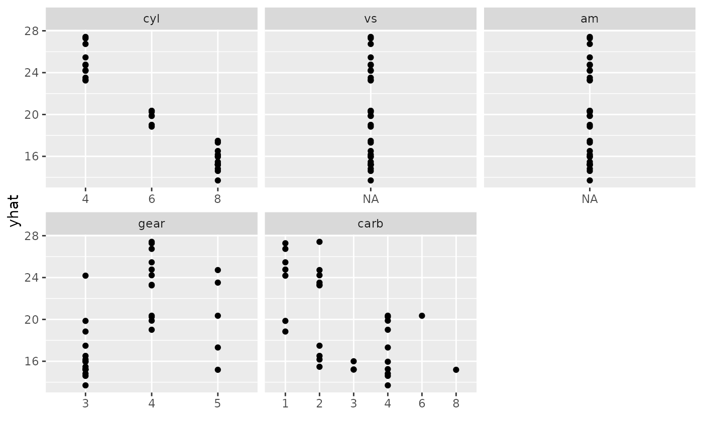
 plot(gg_dta,
xvar = c("cyl", "vs", "am", "gear", "carb"), panel = TRUE,
notch = TRUE
)
#> Warning: attributes are not identical across measure variables; they will be dropped
#> Warning: Ignoring unknown parameters: `notch`
#> Warning: Ignoring unknown parameters: `notch`
#> `geom_smooth()` using method = 'loess' and formula = 'y ~ x'
plot(gg_dta,
xvar = c("cyl", "vs", "am", "gear", "carb"), panel = TRUE,
notch = TRUE
)
#> Warning: attributes are not identical across measure variables; they will be dropped
#> Warning: Ignoring unknown parameters: `notch`
#> Warning: Ignoring unknown parameters: `notch`
#> `geom_smooth()` using method = 'loess' and formula = 'y ~ x'
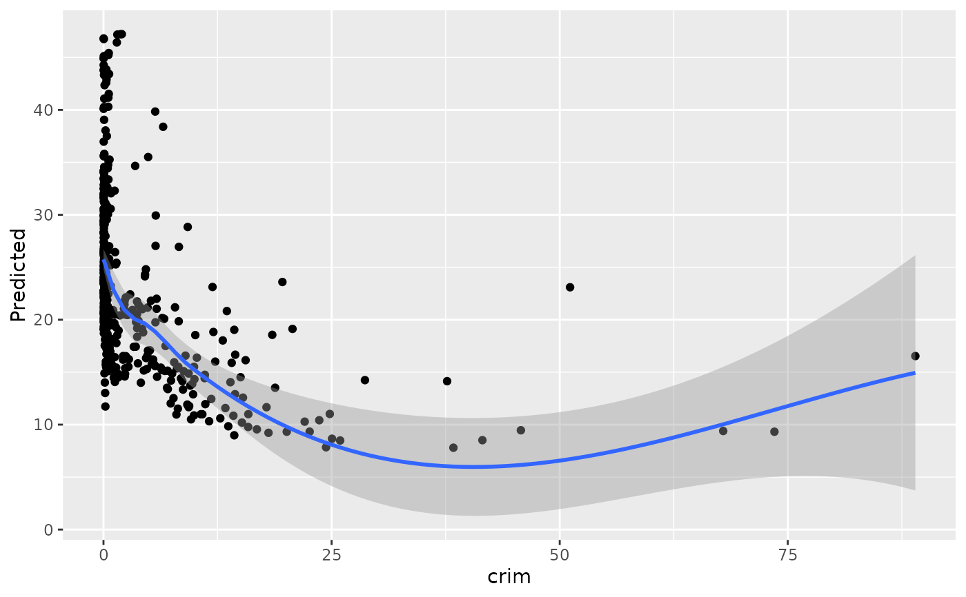
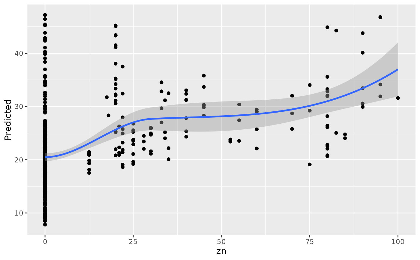
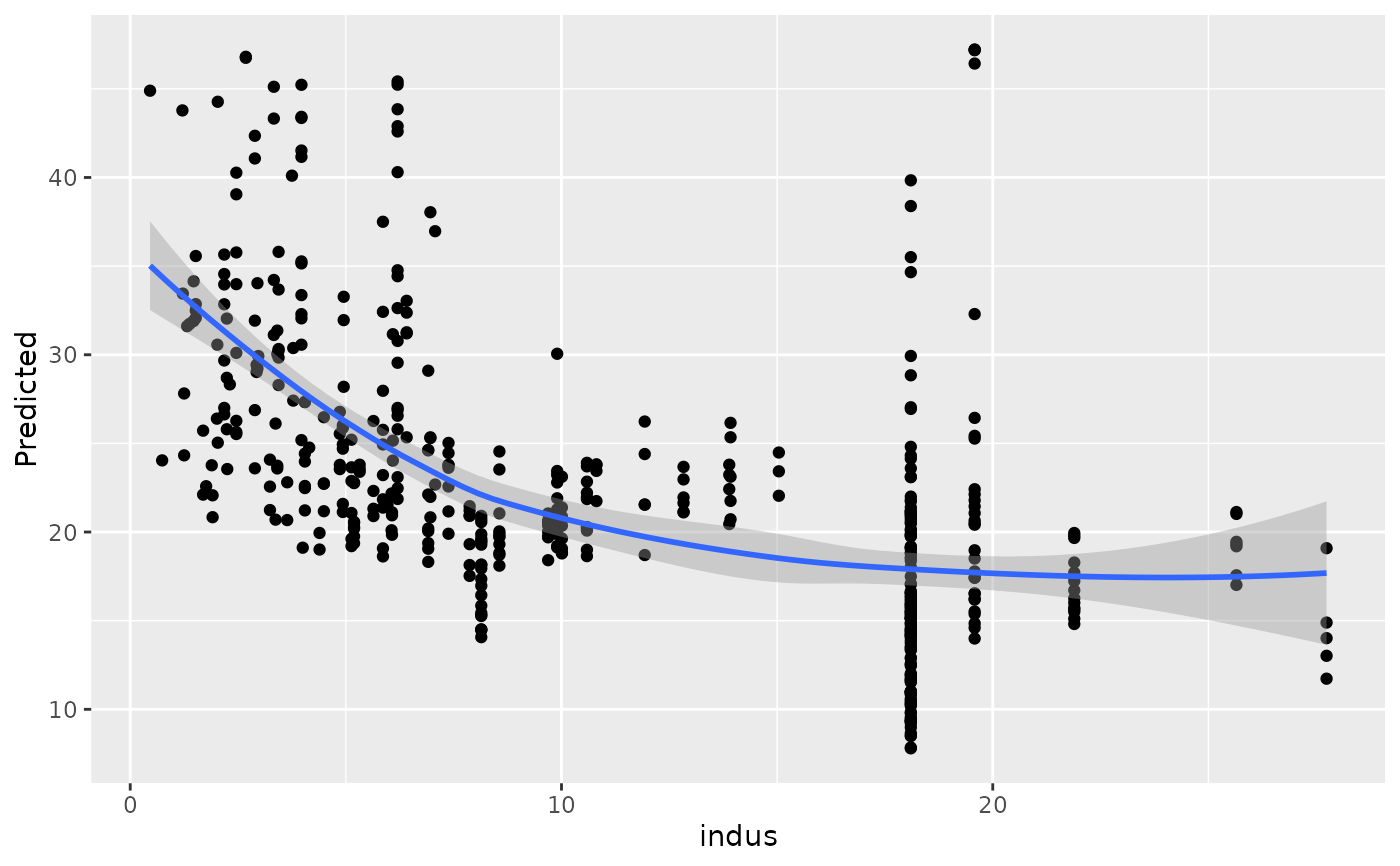
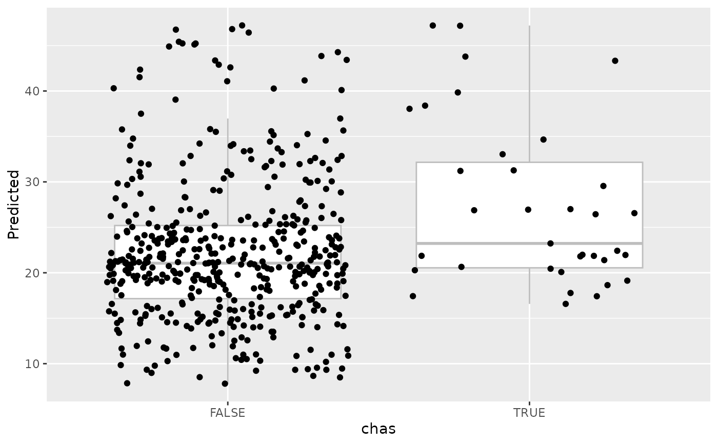
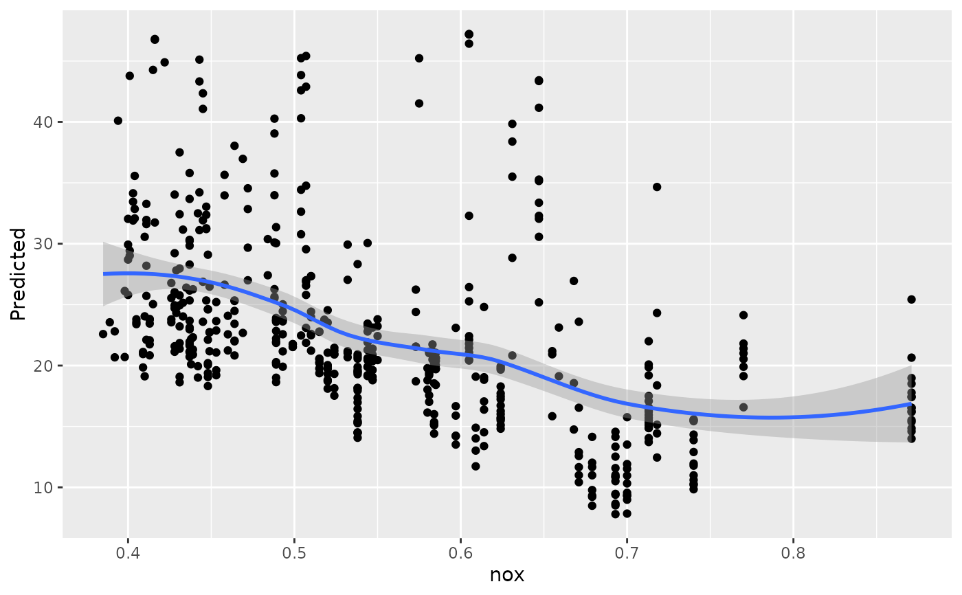
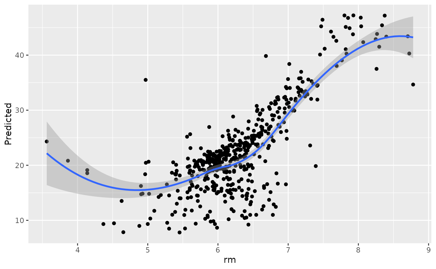
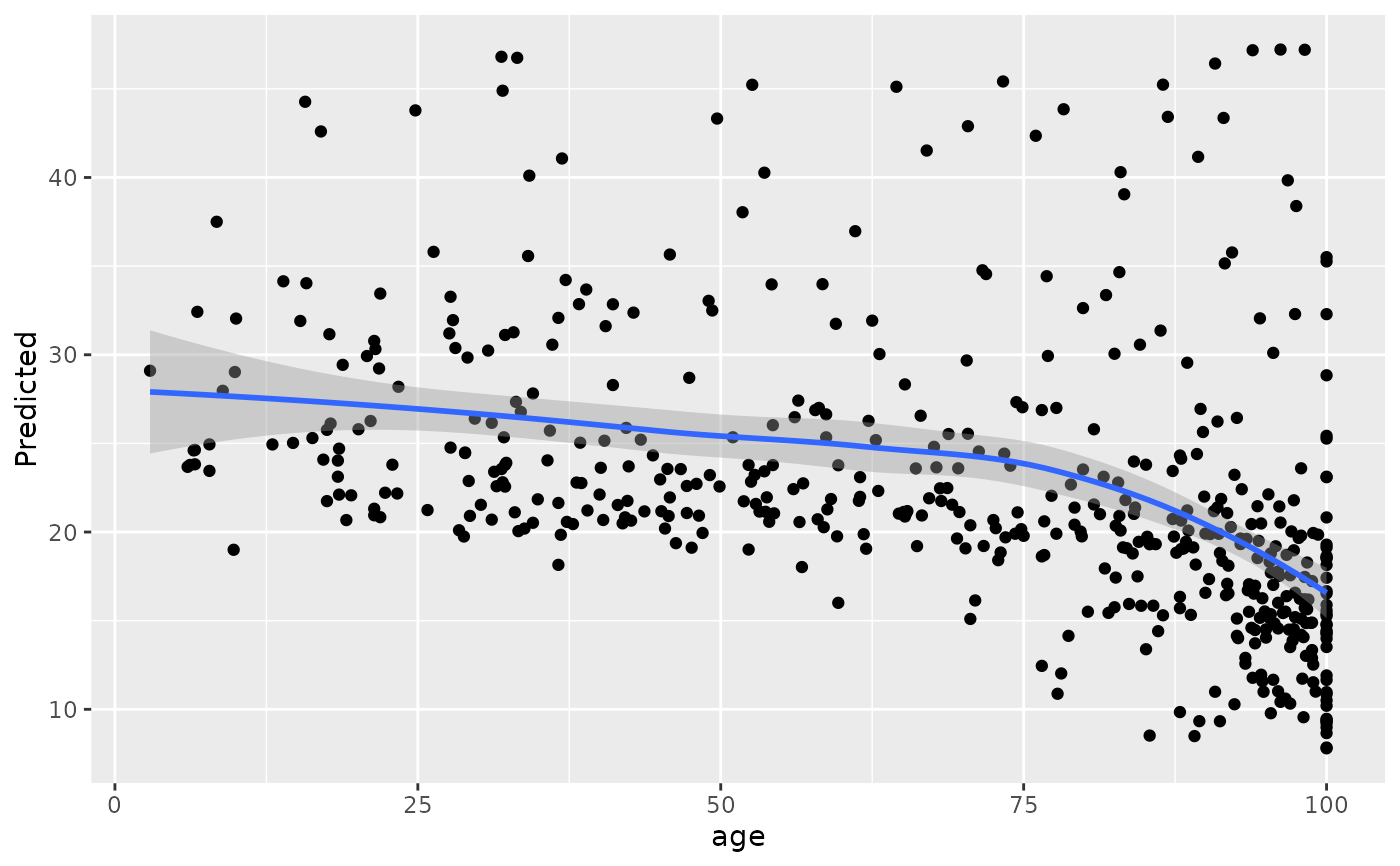
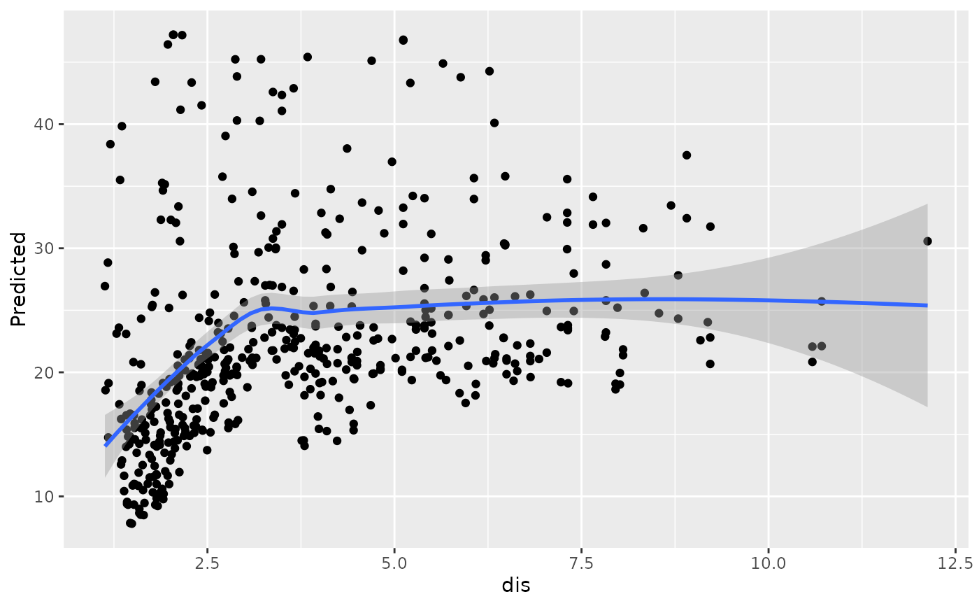
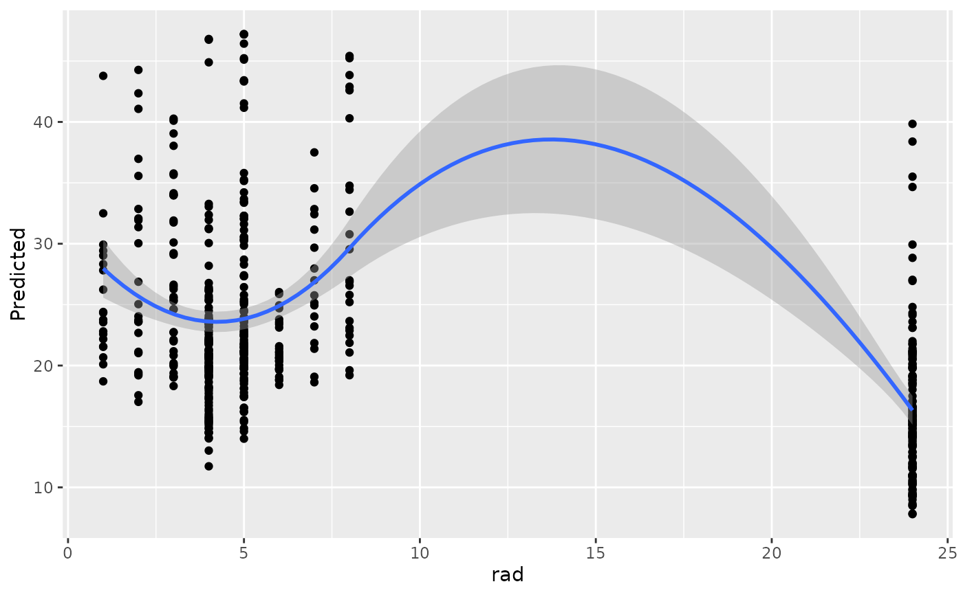
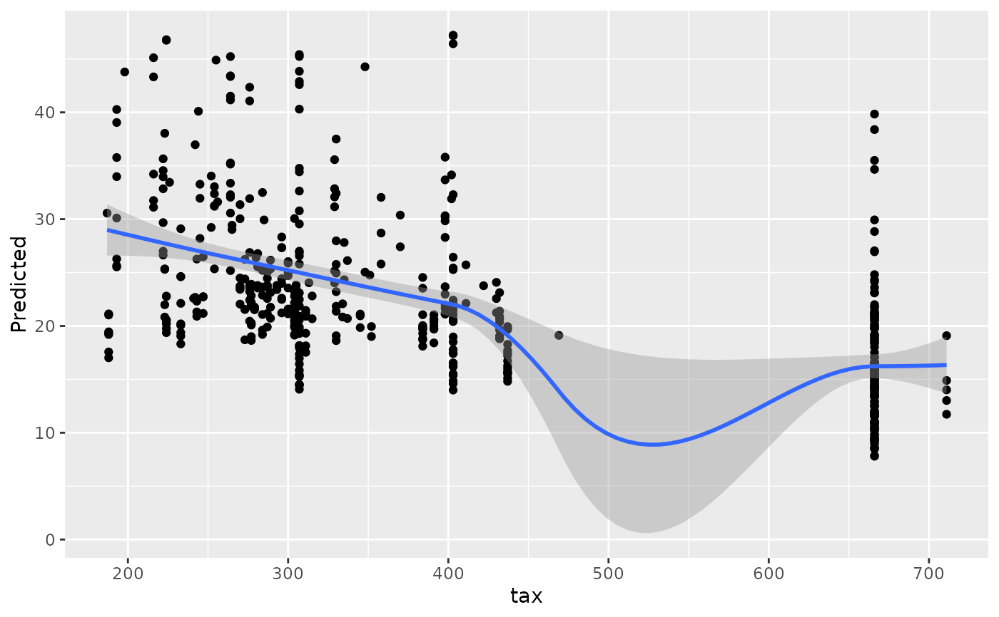
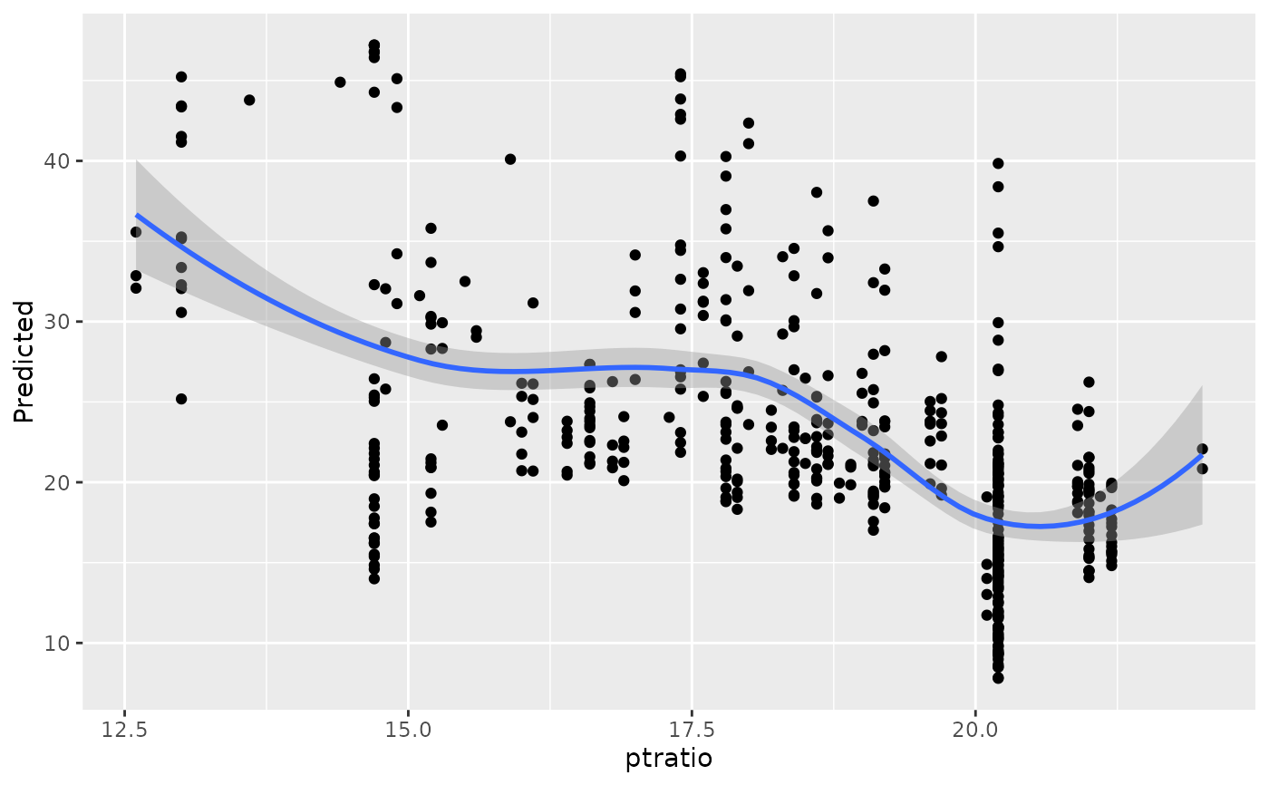
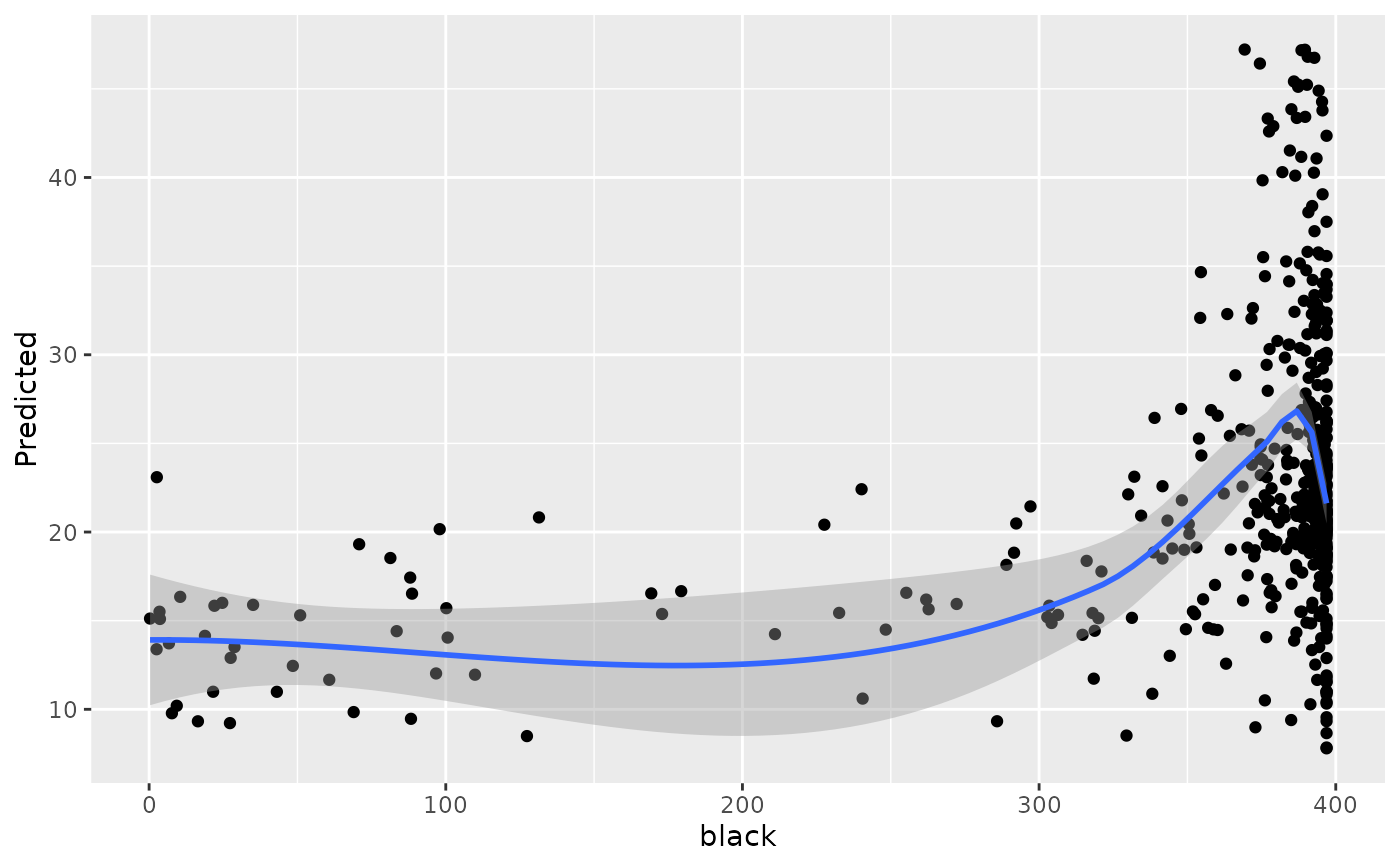
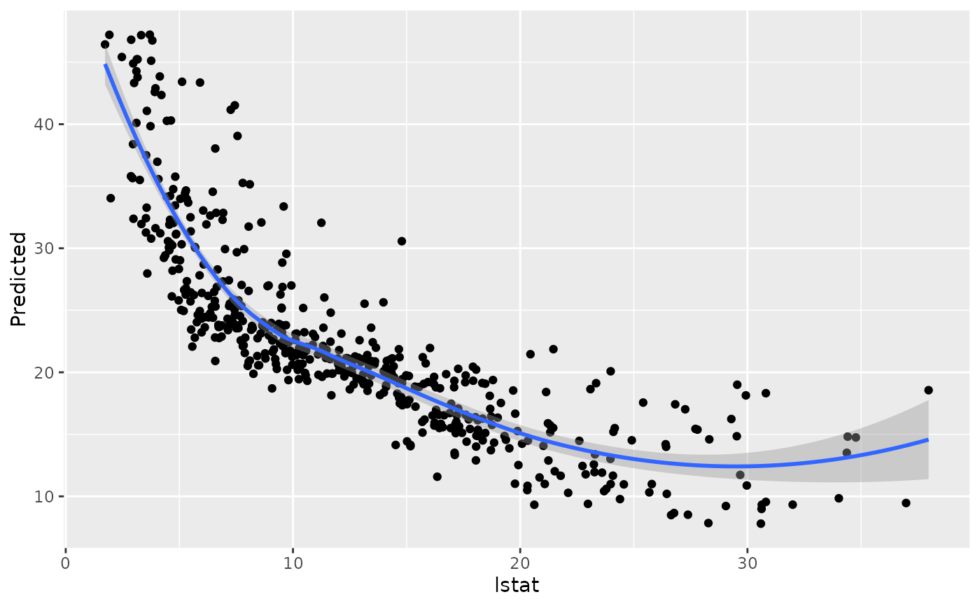
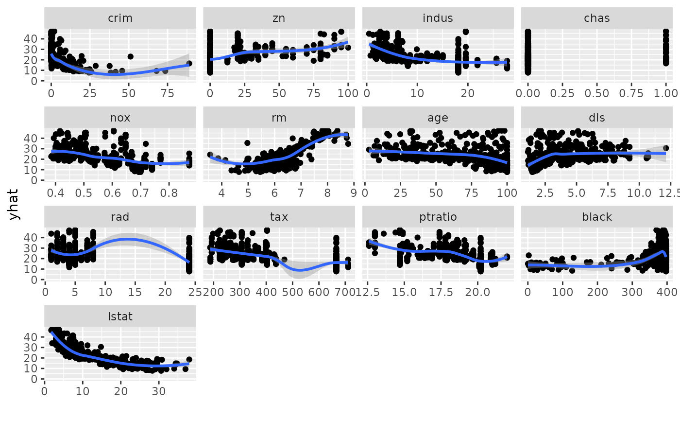
 ## -------- Boston data
data(Boston, package = "MASS")
rf_boston <- randomForest::randomForest(medv ~ ., data = Boston)
gg_dta <- gg_variable(rf_boston)
plot(gg_dta)
#> [[1]]
#> `geom_smooth()` using method = 'loess' and formula = 'y ~ x'
## -------- Boston data
data(Boston, package = "MASS")
rf_boston <- randomForest::randomForest(medv ~ ., data = Boston)
gg_dta <- gg_variable(rf_boston)
plot(gg_dta)
#> [[1]]
#> `geom_smooth()` using method = 'loess' and formula = 'y ~ x'
 #>
#> [[2]]
#> `geom_smooth()` using method = 'loess' and formula = 'y ~ x'
#> Warning: pseudoinverse used at -0.5
#> Warning: neighborhood radius 13
#> Warning: reciprocal condition number 0
#> Warning: There are other near singularities as well. 156.25
#> Warning: pseudoinverse used at -0.5
#> Warning: neighborhood radius 13
#> Warning: reciprocal condition number 0
#> Warning: There are other near singularities as well. 156.25
#>
#> [[2]]
#> `geom_smooth()` using method = 'loess' and formula = 'y ~ x'
#> Warning: pseudoinverse used at -0.5
#> Warning: neighborhood radius 13
#> Warning: reciprocal condition number 0
#> Warning: There are other near singularities as well. 156.25
#> Warning: pseudoinverse used at -0.5
#> Warning: neighborhood radius 13
#> Warning: reciprocal condition number 0
#> Warning: There are other near singularities as well. 156.25
 #>
#> [[3]]
#> `geom_smooth()` using method = 'loess' and formula = 'y ~ x'
#>
#> [[3]]
#> `geom_smooth()` using method = 'loess' and formula = 'y ~ x'
 #>
#> [[4]]
#>
#> [[4]]
 #>
#> [[5]]
#> `geom_smooth()` using method = 'loess' and formula = 'y ~ x'
#>
#> [[5]]
#> `geom_smooth()` using method = 'loess' and formula = 'y ~ x'
 #>
#> [[6]]
#> `geom_smooth()` using method = 'loess' and formula = 'y ~ x'
#>
#> [[6]]
#> `geom_smooth()` using method = 'loess' and formula = 'y ~ x'
 #>
#> [[7]]
#> `geom_smooth()` using method = 'loess' and formula = 'y ~ x'
#>
#> [[7]]
#> `geom_smooth()` using method = 'loess' and formula = 'y ~ x'
 #>
#> [[8]]
#> `geom_smooth()` using method = 'loess' and formula = 'y ~ x'
#>
#> [[8]]
#> `geom_smooth()` using method = 'loess' and formula = 'y ~ x'
 #>
#> [[9]]
#> `geom_smooth()` using method = 'loess' and formula = 'y ~ x'
#>
#> [[9]]
#> `geom_smooth()` using method = 'loess' and formula = 'y ~ x'
 #>
#> [[10]]
#> `geom_smooth()` using method = 'loess' and formula = 'y ~ x'
#>
#> [[10]]
#> `geom_smooth()` using method = 'loess' and formula = 'y ~ x'
 #>
#> [[11]]
#> `geom_smooth()` using method = 'loess' and formula = 'y ~ x'
#>
#> [[11]]
#> `geom_smooth()` using method = 'loess' and formula = 'y ~ x'
 #>
#> [[12]]
#> `geom_smooth()` using method = 'loess' and formula = 'y ~ x'
#>
#> [[12]]
#> `geom_smooth()` using method = 'loess' and formula = 'y ~ x'
 #>
#> [[13]]
#> `geom_smooth()` using method = 'loess' and formula = 'y ~ x'
#>
#> [[13]]
#> `geom_smooth()` using method = 'loess' and formula = 'y ~ x'
 #>
plot(gg_dta, panel = TRUE)
#> Warning: Mismatched variable types...
#> assuming these are all factor variables.
#> `geom_smooth()` using method = 'loess' and formula = 'y ~ x'
#> Warning: pseudoinverse used at -0.5
#> Warning: neighborhood radius 13
#> Warning: reciprocal condition number 0
#> Warning: There are other near singularities as well. 156.25
#> Warning: pseudoinverse used at -0.5
#> Warning: neighborhood radius 13
#> Warning: reciprocal condition number 0
#> Warning: There are other near singularities as well. 156.25
#> Warning: at -0.005
#> Warning: radius 2.5e-05
#> Warning: all data on boundary of neighborhood. make span bigger
#> Warning: pseudoinverse used at -0.005
#> Warning: neighborhood radius 0.005
#> Warning: reciprocal condition number 1
#> Warning: There are other near singularities as well. 1.01
#> Warning: zero-width neighborhood. make span bigger
#> Warning: Failed to fit group -1.
#> Caused by error in `predLoess()`:
#> ! NA/NaN/Inf in foreign function call (arg 5)
#>
plot(gg_dta, panel = TRUE)
#> Warning: Mismatched variable types...
#> assuming these are all factor variables.
#> `geom_smooth()` using method = 'loess' and formula = 'y ~ x'
#> Warning: pseudoinverse used at -0.5
#> Warning: neighborhood radius 13
#> Warning: reciprocal condition number 0
#> Warning: There are other near singularities as well. 156.25
#> Warning: pseudoinverse used at -0.5
#> Warning: neighborhood radius 13
#> Warning: reciprocal condition number 0
#> Warning: There are other near singularities as well. 156.25
#> Warning: at -0.005
#> Warning: radius 2.5e-05
#> Warning: all data on boundary of neighborhood. make span bigger
#> Warning: pseudoinverse used at -0.005
#> Warning: neighborhood radius 0.005
#> Warning: reciprocal condition number 1
#> Warning: There are other near singularities as well. 1.01
#> Warning: zero-width neighborhood. make span bigger
#> Warning: Failed to fit group -1.
#> Caused by error in `predLoess()`:
#> ! NA/NaN/Inf in foreign function call (arg 5)
 ## ------------------------------------------------------------
## survival examples
## ------------------------------------------------------------
## -------- veteran data
## survival
data(veteran, package = "randomForestSRC")
rfsrc_veteran <- rfsrc(Surv(time, status) ~ ., veteran,
nsplit = 10,
ntree = 100
)
# get the 1 year survival time.
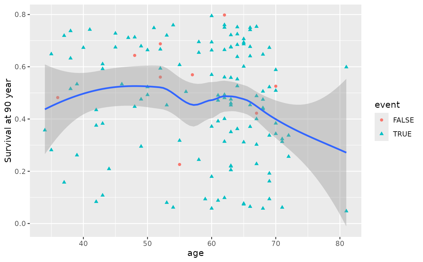
gg_dta <- gg_variable(rfsrc_veteran, time = 90)
# Generate variable dependence plots for age and diagtime
plot(gg_dta, xvar = "age")
#> `geom_smooth()` using method = 'loess' and formula = 'y ~ x'
## ------------------------------------------------------------
## survival examples
## ------------------------------------------------------------
## -------- veteran data
## survival
data(veteran, package = "randomForestSRC")
rfsrc_veteran <- rfsrc(Surv(time, status) ~ ., veteran,
nsplit = 10,
ntree = 100
)
# get the 1 year survival time.
gg_dta <- gg_variable(rfsrc_veteran, time = 90)
# Generate variable dependence plots for age and diagtime
plot(gg_dta, xvar = "age")
#> `geom_smooth()` using method = 'loess' and formula = 'y ~ x'
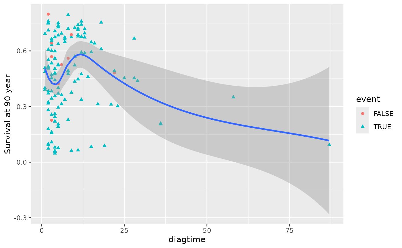
 plot(gg_dta, xvar = "diagtime", )
#> `geom_smooth()` using method = 'loess' and formula = 'y ~ x'
plot(gg_dta, xvar = "diagtime", )
#> `geom_smooth()` using method = 'loess' and formula = 'y ~ x'
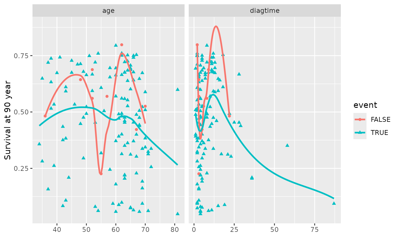
 # Generate coplots
plot(gg_dta, xvar = c("age", "diagtime"), panel = TRUE, se = FALSE)
#> Warning: Ignoring unknown parameters: `se`
#> `geom_smooth()` using method = 'loess' and formula = 'y ~ x'
# Generate coplots
plot(gg_dta, xvar = c("age", "diagtime"), panel = TRUE, se = FALSE)
#> Warning: Ignoring unknown parameters: `se`
#> `geom_smooth()` using method = 'loess' and formula = 'y ~ x'
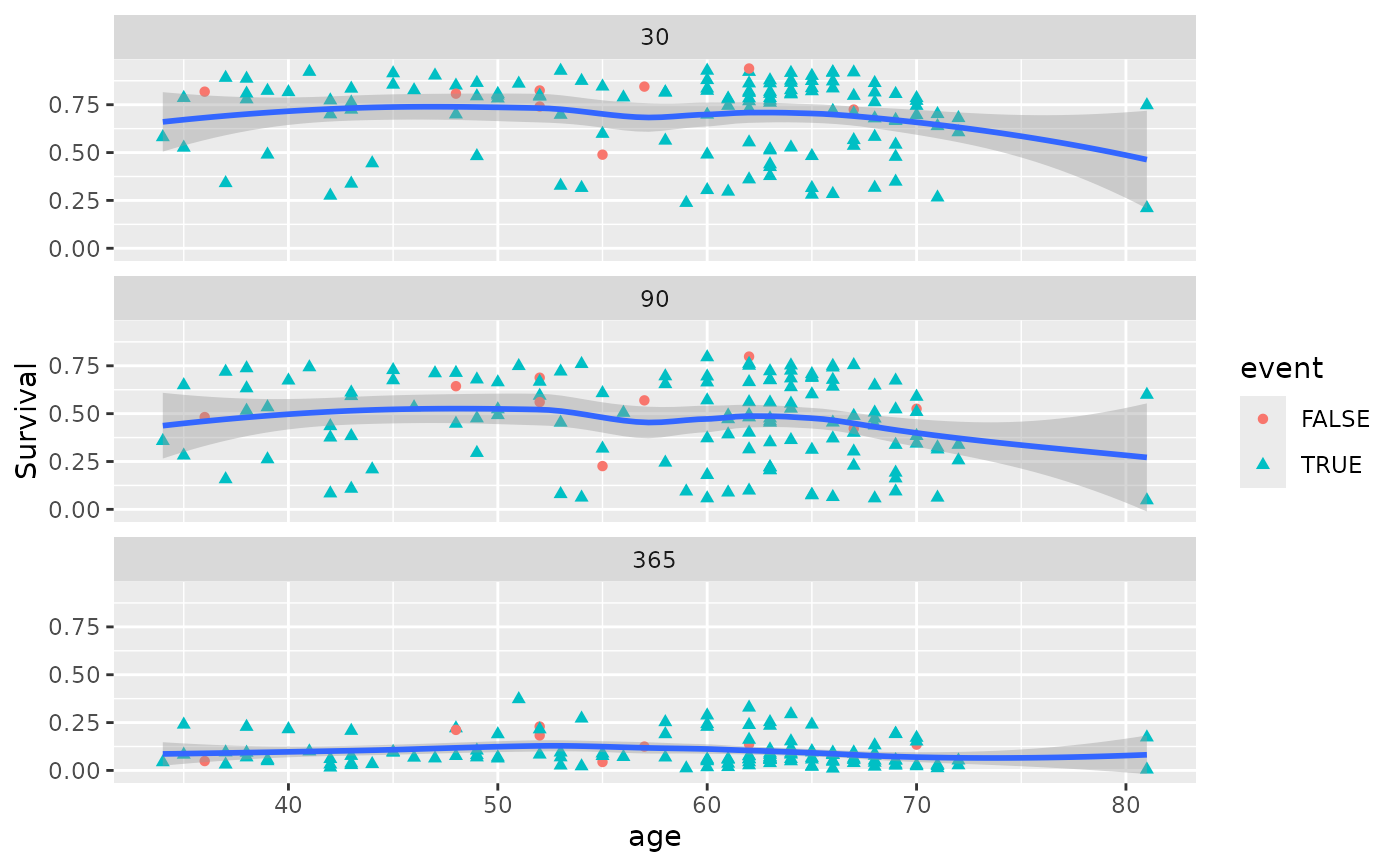
 # If we want to compare survival at different time points, say 30, 90 day
# and 1 year
gg_dta <- gg_variable(rfsrc_veteran, time = c(30, 90, 365))
# Generate variable dependence plots for age and diagtime
plot(gg_dta, xvar = "age")
#> `geom_smooth()` using method = 'loess' and formula = 'y ~ x'
# If we want to compare survival at different time points, say 30, 90 day
# and 1 year
gg_dta <- gg_variable(rfsrc_veteran, time = c(30, 90, 365))
# Generate variable dependence plots for age and diagtime
plot(gg_dta, xvar = "age")
#> `geom_smooth()` using method = 'loess' and formula = 'y ~ x'
 ## -------- pbc data
## We don't run this because of bootstrap confidence limits
# We need to create this dataset
data(pbc, package = "randomForestSRC", )
#> Warning: data set ‘’ not found
# For whatever reason, the age variable is in days... makes no sense to me
for (ind in seq_len(dim(pbc)[2])) {
if (!is.factor(pbc[, ind])) {
if (length(unique(pbc[which(!is.na(pbc[, ind])), ind])) <= 2) {
if (sum(range(pbc[, ind], na.rm = TRUE) == c(0, 1)) == 2) {
pbc[, ind] <- as.logical(pbc[, ind])
}
}
} else {
if (length(unique(pbc[which(!is.na(pbc[, ind])), ind])) <= 2) {
if (sum(sort(unique(pbc[, ind])) == c(0, 1)) == 2) {
pbc[, ind] <- as.logical(pbc[, ind])
}
if (sum(sort(unique(pbc[, ind])) == c(FALSE, TRUE)) == 2) {
pbc[, ind] <- as.logical(pbc[, ind])
}
}
}
if (!is.logical(pbc[, ind]) &
length(unique(pbc[which(!is.na(pbc[, ind])), ind])) <= 5) {
pbc[, ind] <- factor(pbc[, ind])
}
}
# Convert age to years
pbc$age <- pbc$age / 364.24
pbc$years <- pbc$days / 364.24
pbc <- pbc[, -which(colnames(pbc) == "days")]
pbc$treatment <- as.numeric(pbc$treatment)
pbc$treatment[which(pbc$treatment == 1)] <- "DPCA"
pbc$treatment[which(pbc$treatment == 2)] <- "placebo"
pbc$treatment <- factor(pbc$treatment)
dta_train <- pbc[-which(is.na(pbc$treatment)), ]
# Create a test set from the remaining patients
pbc_test <- pbc[which(is.na(pbc$treatment)), ]
# ========
# build the forest:
rfsrc_pbc <- randomForestSRC::rfsrc(
Surv(years, status) ~ .,
dta_train,
nsplit = 10,
na.action = "na.impute",
forest = TRUE,
importance = TRUE,
save.memory = TRUE
)
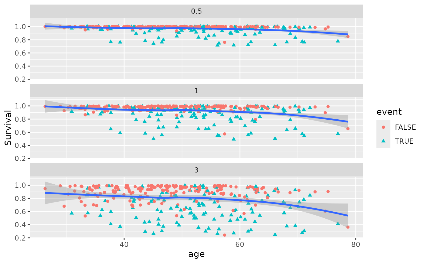
gg_dta <- gg_variable(rfsrc_pbc, time = c(.5, 1, 3))
plot(gg_dta, xvar = "age")
#> `geom_smooth()` using method = 'loess' and formula = 'y ~ x'
## -------- pbc data
## We don't run this because of bootstrap confidence limits
# We need to create this dataset
data(pbc, package = "randomForestSRC", )
#> Warning: data set ‘’ not found
# For whatever reason, the age variable is in days... makes no sense to me
for (ind in seq_len(dim(pbc)[2])) {
if (!is.factor(pbc[, ind])) {
if (length(unique(pbc[which(!is.na(pbc[, ind])), ind])) <= 2) {
if (sum(range(pbc[, ind], na.rm = TRUE) == c(0, 1)) == 2) {
pbc[, ind] <- as.logical(pbc[, ind])
}
}
} else {
if (length(unique(pbc[which(!is.na(pbc[, ind])), ind])) <= 2) {
if (sum(sort(unique(pbc[, ind])) == c(0, 1)) == 2) {
pbc[, ind] <- as.logical(pbc[, ind])
}
if (sum(sort(unique(pbc[, ind])) == c(FALSE, TRUE)) == 2) {
pbc[, ind] <- as.logical(pbc[, ind])
}
}
}
if (!is.logical(pbc[, ind]) &
length(unique(pbc[which(!is.na(pbc[, ind])), ind])) <= 5) {
pbc[, ind] <- factor(pbc[, ind])
}
}
# Convert age to years
pbc$age <- pbc$age / 364.24
pbc$years <- pbc$days / 364.24
pbc <- pbc[, -which(colnames(pbc) == "days")]
pbc$treatment <- as.numeric(pbc$treatment)
pbc$treatment[which(pbc$treatment == 1)] <- "DPCA"
pbc$treatment[which(pbc$treatment == 2)] <- "placebo"
pbc$treatment <- factor(pbc$treatment)
dta_train <- pbc[-which(is.na(pbc$treatment)), ]
# Create a test set from the remaining patients
pbc_test <- pbc[which(is.na(pbc$treatment)), ]
# ========
# build the forest:
rfsrc_pbc <- randomForestSRC::rfsrc(
Surv(years, status) ~ .,
dta_train,
nsplit = 10,
na.action = "na.impute",
forest = TRUE,
importance = TRUE,
save.memory = TRUE
)
gg_dta <- gg_variable(rfsrc_pbc, time = c(.5, 1, 3))
plot(gg_dta, xvar = "age")
#> `geom_smooth()` using method = 'loess' and formula = 'y ~ x'
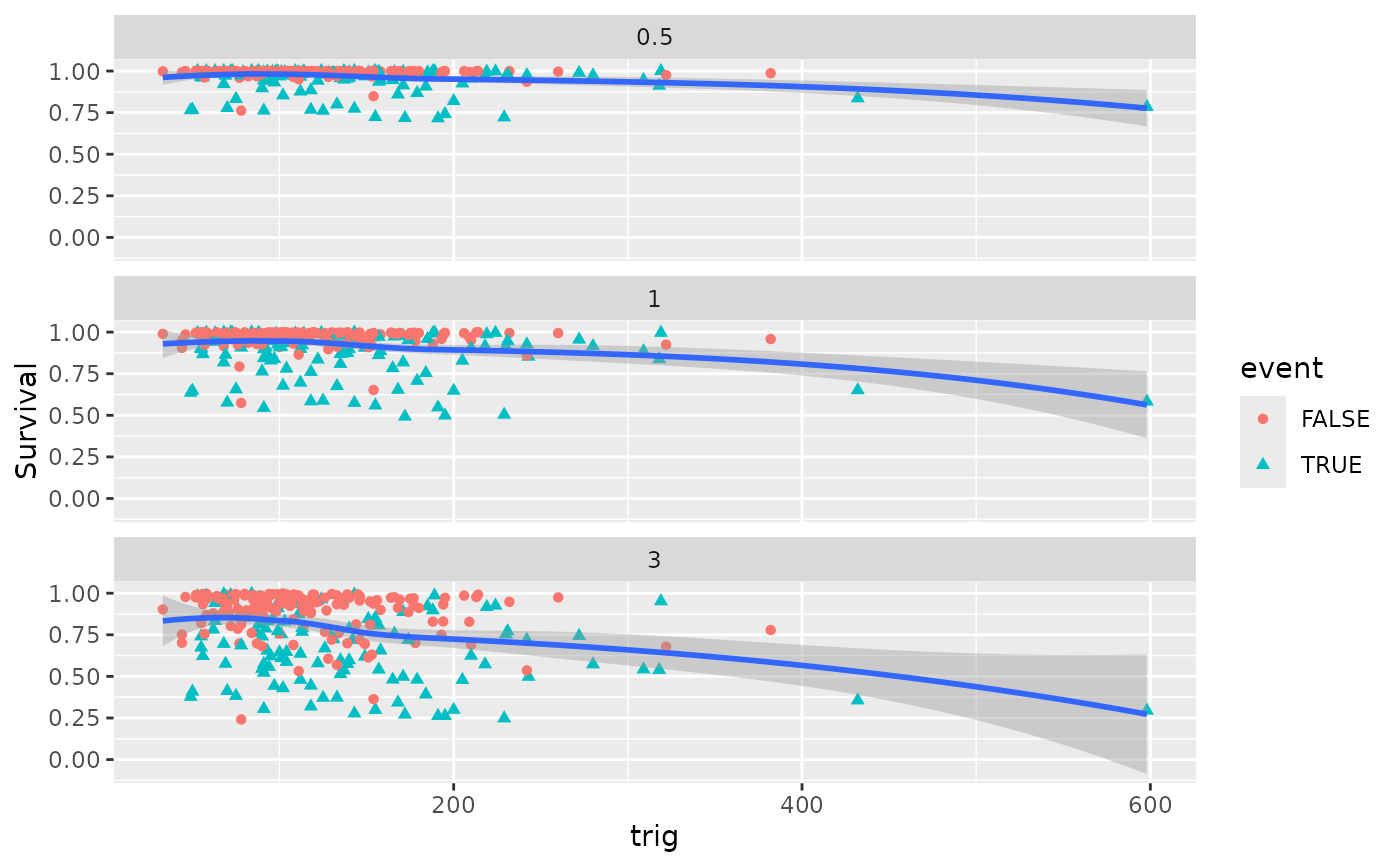
 plot(gg_dta, xvar = "trig")
#> `geom_smooth()` using method = 'loess' and formula = 'y ~ x'
#> Warning: Removed 90 rows containing non-finite outside the scale range
#> (`stat_smooth()`).
#> Warning: Removed 90 rows containing missing values or values outside the scale range
#> (`geom_point()`).
plot(gg_dta, xvar = "trig")
#> `geom_smooth()` using method = 'loess' and formula = 'y ~ x'
#> Warning: Removed 90 rows containing non-finite outside the scale range
#> (`stat_smooth()`).
#> Warning: Removed 90 rows containing missing values or values outside the scale range
#> (`geom_point()`).
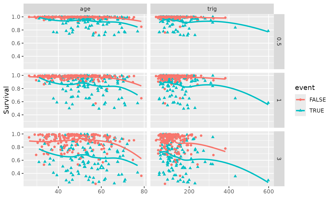
 # Generate coplots
plot(gg_dta, xvar = c("age", "trig"), panel = TRUE, se = FALSE)
#> Warning: Ignoring unknown parameters: `se`
#> `geom_smooth()` using method = 'loess' and formula = 'y ~ x'
#> Warning: Removed 90 rows containing non-finite outside the scale range
#> (`stat_smooth()`).
#> Warning: Removed 90 rows containing missing values or values outside the scale range
#> (`geom_point()`).
# Generate coplots
plot(gg_dta, xvar = c("age", "trig"), panel = TRUE, se = FALSE)
#> Warning: Ignoring unknown parameters: `se`
#> `geom_smooth()` using method = 'loess' and formula = 'y ~ x'
#> Warning: Removed 90 rows containing non-finite outside the scale range
#> (`stat_smooth()`).
#> Warning: Removed 90 rows containing missing values or values outside the scale range
#> (`geom_point()`).