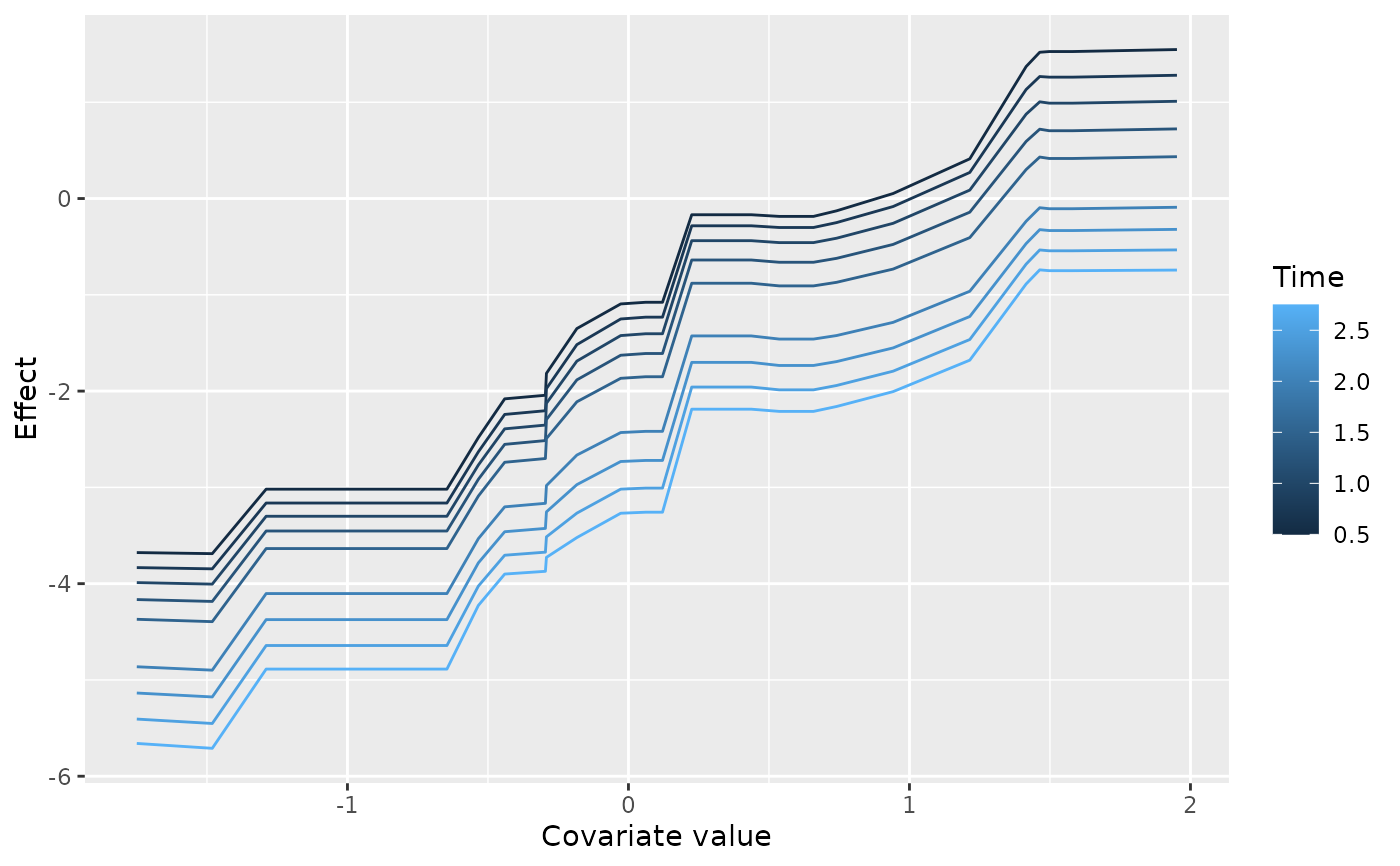
Covariate effect curves, one line per time point, faceted by variable and, for a multi-response fit, by response.
Usage
# S3 method for class 'gg_boost_effect'
autoplot(object, ...)

# S3 method for class 'gg_boost_effect'
plot(x, ...)
Arguments
- object
A
gg_boost_effectobject.- ...
Passed to
geom_line(continuous covariates) orgeom_point(discrete covariates).- x
A
gg_boost_effectobject.
Details
Time is mapped to colour rather than to a facet because the question this figure answers is how a covariate's effect changes across follow-up, and that change is legible only when the curves share one panel. Variables get the facets instead, since their x scales are unrelated.
A continuous covariate is drawn as a line per time point across the
covariate grid. A discrete (factor) covariate has one row per level, so
a "curve" would connect points along an axis with no ordering; it is
drawn instead as a point per level per time point, on an axis labelled
with the level names. Because ggplot2 permits only one scale type per
aesthetic across all facets, an object mixing continuous and discrete
covariates cannot be drawn as a single figure and is refused with an
error asking the caller to plot them one at a time.
The returned plot carries no theme.
Examples
# \donttest{
sim <- boostmtree::simLong(n = 25, n.time = 4, model = 1)$data.list
fit <- boostmtree::boostmtree(
x = sim$features, tm = sim$time, id = sim$id, y = sim$y,
M = 50, verbose = FALSE
)
pp <- boostmtree::partial.plot(
fit, x.var.names = "x1", output = "data", verbose = FALSE
)
plot(gg_boost_effect(pp))
 # }