Extract covariate effect curves over time from a
partial.plot or
marginal.plot object, or from the
boostmlr_partial result for a BoostMLR fit.
Arguments
- object
A
partial.plot.boostmtreeormarginal.plot.boostmtreeobject, as returned byboostmtree::partial.plot()orboostmtree::marginal.plot()withoutput = "data", verbose = FALSE, or aboostmlr_partialobject.- ...
Not used; present for S3 consistency.
Value
A gg_boost_effect data.frame with columns:
- variable
Factor covariate name.
- x
Numeric covariate value. For a continuous covariate this is the covariate itself; for a discrete (factor) covariate this is an integer position, one per level.
- x_label
Character level label for a discrete covariate,
NAfor a continuous one.- time
Numeric time point.
- estimate
Numeric fitted effect.
- kind
Factor,
partialormarginal.- response
Factor naming the response.
Details
The two differ in what they hold constant. A partial effect varies one
covariate while averaging over the others; a marginal effect reads the fitted
surface as the data actually distribute it. Both are covariate-by-time
surfaces, so both land in this one class, distinguished by kind.
marginal.plot() returns a raw scatter alongside its smoothed curve.
That scatter is not the raw observations: it holds one unsmoothed fitted
prediction per subject at the subject's own observed covariate value,
not the observed response and not the stored fitted values. It is also
not reconstructable from gg_boost_trajectory, which carries
no covariate column. gg_boost_effect extracts the smoothed curve instead,
so that both levels of kind mean the same thing: the fitted effect.
For BoostMLR, boostmlr_partial returns both the raw
partial effect and a lowess smooth of it over time; the smooth is
extracted, matching the marginal choice above. The result has kind
partial and one block per response, labelled from the fit's y_Names.
No source computes a confidence interval, so none is reported here.
boostmtree accepts factor covariates. For those, partial.plot() and
marginal.plot() return a character (or, for marginal.plot()$data,
factor) x column with one row per level rather than a numeric grid.
gg_boost_effect detects this and maps each level to an integer position
in x, carrying the level itself in x_label; a continuous covariate
keeps its numeric value in x and leaves x_label NA. The grid is
resolved once per variable so every time point shares the same level
ordering.
A multi-response fit (family = "ordinal" or "nominal") nests
$curves / $smooth as [[response]][[variable]]; a single-response fit
flattens the outer level. gg_boost_effect accepts both and records the
response in a response column, labelled from the object's
$response.labels ("response" for a single-response fit). Each response
of an ordinal or nominal fit is one model component, so its curves are on
that component's scale.
Examples
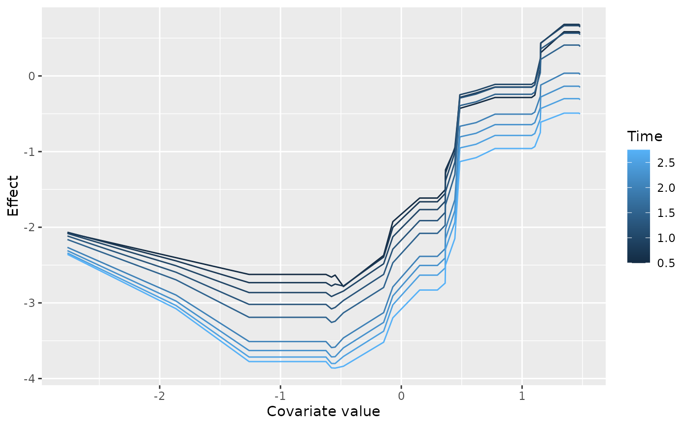
# \donttest{
sim <- boostmtree::simLong(n = 25, n.time = 4, model = 1)$data.list
fit <- boostmtree::boostmtree(
x = sim$features, tm = sim$time, id = sim$id, y = sim$y,
M = 50, verbose = FALSE
)
pp <- boostmtree::partial.plot(
fit, x.var.names = "x1", output = "data", verbose = FALSE
)
plot(gg_boost_effect(pp))
 # }