Plot a gg_boost_trajectory object

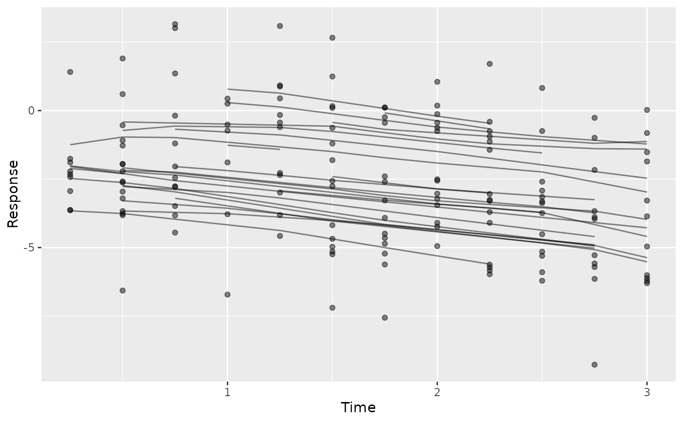
Observed and fitted subject trajectories over time: one line per subject through the fitted values, with the observed values as points.

Usage

# S3 method for class 'gg_boost_trajectory'
autoplot(
  object,
  subset = NULL,
  n_max = 100,
  observed = TRUE,
  alpha = NULL,
  ...
)

# S3 method for class 'gg_boost_trajectory'
plot(x, subset = NULL, n_max = 100, observed = TRUE, alpha = NULL, ...)

Arguments

object

A gg_boost_trajectory object.

subset

Character or numeric vector of subject identifiers to keep. NULL (default) keeps all of them.

n_max

Maximum number of subjects to draw. Defaults to 100; Inf draws every subject.

observed

Logical. Draw the observed values as points. Defaults to TRUE, and is ignored when the fit records no observed values.

alpha

Numeric transparency for both layers. NULL (default) computes one from the number of subjects drawn.

...

Passed to geom_line.

x

A gg_boost_trajectory object.

Value

A ggplot object.

Details

The extractor returns every subject, so thinning happens here and the tidy data frame always represents the whole fit. subset names the subjects to keep; n_max caps how many are drawn, sampling at random and saying so. Set n_max = Inf to draw all of them. Random sampling is not seeded – call set.seed() first for a reproducible figure.

Transparency is doing real work in this figure rather than decorating it. A cohort of any size overplots, and partial transparency turns the tangle into something you can read densities off: where many subjects follow the same path the ink accumulates. The default alpha therefore falls as the number of subjects drawn rises. Pass alpha explicitly to override.

The returned plot carries no theme.

See also

gg_boost_trajectory

Examples

# \donttest{
sim <- boostmtree::simLong(n = 25, n.time = 4, model = 1)$data.list
fit <- boostmtree::boostmtree(
  x = sim$features, tm = sim$time, id = sim$id, y = sim$y,
  M = 50, verbose = FALSE
)
plot(gg_boost_trajectory(fit))

# }