Calibration over follow-up data object

Compare observed and fitted values over follow-up time, binned by time, with an optional cohort mean curve.

Usage

gg_boost_calibration(object, pred = NULL, n_bins = 10, breaks = NULL, ...)

Arguments

object

A fitted boostmtree object, or a fitted BoostMLR object. Not a predict object: pass that as pred.

pred

Optional boostmtree predict object from predict(fit, x = ...), used for the cohort curve.

n_bins

Number of equal-count time bins. Defaults to 10.

breaks

Optional numeric vector of bin edges in the fit's time units. Overrides n_bins.

...

Not used; present for S3 consistency.

Value

A gg_boost_calibration data.frame with one row per response and bin, ordered by response then time, with columns:

response

Factor naming the response.

bin

Factor bin label, ordered by time within each response.

time_lo, time_hi

Numeric bin edges.

time

Numeric median observed time within the bin.

n_obs

Integer count of observations in the bin.

n_subject

Integer count of distinct subjects in the bin.

observed

Numeric mean observed value.

observed_lo, observed_hi

Numeric 95\ NA when the bin holds one observation.

fitted

Numeric mean fitted value at the same observations.

When pred is supplied, the attribute cohort holds a data.frame with columns response (factor), time and fitted (numeric).

Details

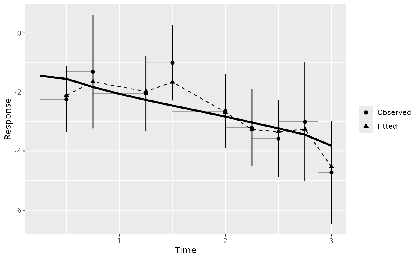
A cohort's predicted curves say what the model expects; they cannot say whether it matches the data. This figure answers that. Observations are binned by time, and each bin reports the mean observed value, the mean fitted value at the same observations, and how many observations and distinct subjects stand behind it.

Bins hold roughly equal numbers of observations by default: the edges are quantiles of observed time, computed per response. Tied times, common in clinical data where many measurements share a visit time, merge quantile edges; duplicates are removed and a message says how many bins survived. Supply breaks, in the fit's own time units, to choose the edges yourself. Observations outside the range of breaks are dropped, with a message giving the count.

With equal-count bins, n_obs is nearly constant by construction, so it cannot show where data thins out. Two columns can: bin width (time_hi - time_lo), which grows where observations are sparse, and n_subject, which falls when a late bin rests on repeat measurements of a few subjects.

The interval on observed is a normal approximation that treats observations as independent. Repeated measurements within a subject make it too narrow. Read it as a visual guide, not an inferential claim.

Supplying pred adds the cohort curve: the mean over subjects of the predicted curves on a common time grid, attached as the cohort attribute. Make pred with predict(fit, x = ...) and no tm or id; with them, each subject is predicted at its own times and a mean across subjects changes composition from one time to the next. The cohort curve is available for boostmtree fits only.

This figure accepts either a boostmtree or a BoostMLR grow fit. It reads its rows from gg_boost_trajectory, so both backends' storage layouts are handled there.

See also

plot.gg_boost_calibration, gg_boost_trajectory

Examples

# \donttest{
sim <- boostmtree::simLong(n = 25, n.time = 4, model = 1)$data.list
fit <- boostmtree::boostmtree(
  x = sim$features, tm = sim$time, id = sim$id, y = sim$y,
  M = 50, verbose = FALSE
)
pred <- predict(fit, x = fit$x)
gg <- gg_boost_calibration(fit, pred = pred)
#> gg_boost_calibration: tied times left 9 of 10 bins for response 'y'.
plot(gg)


# The predicted curves themselves, for a look at who drives the tail:
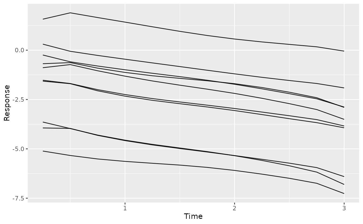
plot(gg_boost_trajectory(pred), n_max = 10)
#> Drawing 10 of 25 subjects, chosen at random. Pass n_max = Inf to draw all, or subset to choose; call set.seed() first for a reproducible sample.

# }