Creates a hazard object and optionally fits it via maximum likelihood.
This mirrors the argument-oriented workflow of the legacy HAZARD C/SAS
implementation: supply starting values in theta and the function will
optimize to produce fitted estimates.
Arguments
- formula
Optional formula with a
Surv()object on the left. Right-censored (Surv(time, status)), left-censored (Surv(time, event, type = "left")), interval-censored (type = "interval"or"interval2") and counting-process (Surv(start, stop, event)) forms are all accepted.Surv()codes censoring status with different integers than this package does; the formula path translates them, so writeSurv()'s codes here. A plainstatusvector takes this package's codes; aSurvpassed asstatusis translated the same way as here. Every distribution carries its own intercept: its baseline parameter, the one the covariates add to, already plays that role, so the design never has one: removing it (~ 0 + age,~ age - 1) is ignored with a warning, and builds the design of~ age. A.on the right-hand side stands for every column ofdatathat theSurv()term does not use, as insurvival::coxph(). When provided, overrides direct time/status/x arguments and extracts from data. Example:hazard(Surv(time, status) ~ x1 + x2, data = df, dist = "weibull", fit = TRUE).- data
Optional data frame. On the formula path it supplies the model frame, and
weightsis evaluated in its scope. On the vector pathtime,status,time_lower,time_upperandweightsare evaluated in its scope, the waybase::subset()andbase::transform()do: a bare column name resolves to that column, and anything that is not a column (df$col, a local vector, a literal) falls through to the calling environment. A column of the same name as a caller variable wins, and because that silently discards the caller's vector (the way a wrapper forwarding its own argument by name does), such a name raises a warning naming the symbol and the argument. The warning reads the names written in the expression. When the argument is the name alone, it says the column was used. When the name is part of a larger expression, it does not say which value was read: the expression may never evaluate the name (an unused function argument), may rebind it first (a loop variable, an assignment) or may evaluate it somewhere else (with()), and the warning cannot tell. A name chosen at run time, as inget(nm)oreval(as.name(nm)), resolves the same way, column first, as it does instats::lm(), but is not checked; the vector path has behaved so since 1.2.2. No second evaluation is made to compare the two values, because evaluating an expression such asrunif(n)twice gives two different vectors. Masked arguments are validated like any other, so anNAin a masked column errors: anNAcount on the SASICENSORpath reachesweightsand stops with'weights' must be non-negative and finite. A named element ofdatathat is a function is refused, on both paths, asstats::lm()refuses it. Because the mask sits in front of the calling frame, such an element would be called in place of the function an expression names –weights = rep(1, n)calling arepheld indata– and the fit would change with nothing to show for it. An S4 generic and a reference-class generator are functions for this purpose. A list-column of functions is a list, not a function, and is unaffected, as is an element with no name, which no expression can look up – but anNA_character_name is refused, because R binds such an element under the symbol`NA`and a call reaches it. Remove the element: for a vector argument orweights, define the helper in the calling environment; for one used inside theSurv()response, compute the value into adatacolumn first, since the response is evaluated without the formula's environment.- time
Numeric follow-up time vector. A row whose time is 0 is dropped before fitting, whatever its status, as PROC HAZARD drops it (
TIME <= 0is inadmissible there). The time tested is the row's upper bound:timefor an exact or right-censored row,time_upperfor a left- or interval-censored one; a lower bound or entry time of 0 is admissible.hazard()warns with the count (class"hzr_time_zero_dropped"), and every row stored on the fit is what remains.fit$data$dropped_time_zerois the count andfit$data$dropped_time_zero_rowstheir positions among the rows given. On the formula interface the response and design are then built on the retained rows, as if the dropped ones had not been given, so a data-dependent term such asscale(age)uses the retained rows. Two inputs are refused because they cannot follow the rows: a response whose values change once the rows are dropped, such asSurv(time - min(time), status), and a formula that reads a per-row value from outsidedata. That check reads the formula's own variables, so it cannot see inside a function: a helper that indexes a vector from outsidedataby position, such asfunction(a) a + g[seq_along(a)], sees only the retained rows and pairs them with the first elements ofg, so every row after the first dropped one is paired with the wrong value. Only the drop itself is warned about; the mis-pairing is not.stats::lm(subset = )is not a guide here: it evaluates the terms on every row and subsets afterwards, so the same helper pairs correctly there. Put such a vector indata, where it is dropped with its rows. A caller-supplied row-aligned input whose row count differs fromtime's is refused before any row is dropped:xandweightson thetime =/status =interface, anddatawherever a formula reads it row by row. (On the formula interface the design is not the caller's; it is rebuilt from the retained rows ofdata.)- status
Numeric or logical event indicator vector, or a
survival::Surv()object. ASurvis read by itstype, exactly as the formula interface reads it, and atime,time_lowerortime_upperthat disagrees with it is an error.- time_lower
Optional numeric vector whose role depends on
status. Supplying it explicitly is not a no-op.status == 2(interval-censored): the lower bound of the censoring interval, defaulting totime. Everydistreads it this way.status %in% c(0, 1)(right-censored or event): the counting-process entry time when0 < time_lower < time, so the row contributesH(time) - H(time_lower). Everydistreads it this way. A value of0, or equal totime, means no entry time, and leftNULLthe entry time is0.status == -1(left-censored): not used; the bound istime_upper.
time_lower = timeon the status 0 and 1 rows is the mixed-interval layout: exact and right-censored rows carry their own time, and only the status-2 rows carry a real lower bound. A subject cannot enter the risk set after the moment it leaves, sohazard()stops with an error when a status 0 or 1 row hastime_lower > time, as SAS HAZARD rejects a start time after the exit time. It also stops when rows withtime_lower == time > 0sit beside rows with genuine entry times: in counting-process data those are zero-length epochs, whichhzr_repeated_events()can emit and which must be adjusted first.- time_upper
Optional numeric upper bound vector for censoring intervals. Used when
status %in% c(-1, 2); defaults totimeif NULL.- x
Optional design matrix (or data frame coercible to matrix). Unlike
timeand the other vector arguments,xis not data-masked:hazard(data = df, time = tt, x = age)errors withobject 'age' not foundwheretime = ttresolves, so writex = df[["age"]]or use the formula interface.- time_windows
Optional numeric vector of strictly positive cut points for piecewise time-varying coefficients. When provided, each predictor column in
xis expanded into one column per time window so each window gets its own coefficient.- theta
Numeric starting values for optimization: the shape parameters, then one coefficient per column of the design matrix. Required when
fit = TRUEwith a single-distributiondist; optional fordist = "multiphase", which assembles its own starting values fromphaseswhenthetaisNULL.- dist
Character baseline distribution label (default
"weibull"). One of"weibull","exponential","loglogistic","lognormal", or"multiphase". The single-distribution families differ in the shape the hazard traces over time;"multiphase"builds an additive N-phase hazard and requiresphases. See the Baseline distributions section for what each means and when to use it.- phases
Optional named list of
hzr_phase()objects specifying the phases for a multiphase model (dist = "multiphase"). Names must be unique, and"total"and"time"are reserved: they label the summed column and the column of prediction times in the decomposed output ofpredict.hazard(), so a phase of either name is rejected. See Examples.- fit
Logical; if TRUE, fit the model via maximum likelihood (default FALSE).
- weights
Optional numeric vector of observation weights (non-negative). Each observation's log-likelihood contribution is multiplied by its weight. Use for severity-weighted repeated events. Default
NULL(unit weights). Implements the SASWEIGHTstatement. Withdata, a name is looked up among its columns first and then in the calling environment, on both interfaces.stats::lm()also looks indatafirst, but then in the formula's environment rather than the caller's, so a formula built inside another function does not bring that function's variables with it here. Seedatafor the warning raised when a name is both.weightsis evaluated over every row given, so an expression that depends on the rows –weights = w / mean(w)– includes any row later dropped for time 0 (seetime); compute it indataon the rows you intend to fit if that matters.- control
Named list of control options (see Details).
- objective
Which interval-censored contribution the multiphase likelihood accumulates.
"likelihood"(default) uses the interval probability \(\log(S(l) - S(u))\)."sas"reproduces whatPROC HAZARDaccumulates: the event-density term with the instantaneous hazard replaced by the interval-mean hazard over \((l, u]\). Applies only todist = "multiphase"; exact-event and right-censored rows are unaffected either way."sas"requires data it can represent: no left-censored rows (PROC HAZARDhas no left-censoring statement) and a positive width on every interval-censored row (the interval-mean hazard divides by \(u - l\)). Both are properties of the data rather than of the fit, so they are checked when the argument is supplied, including underfit = FALSE, which therefore stops rather than returning an unusable object.- ...
Additional named arguments retained for parity with legacy calling conventions.
Value
An object of class hazard, a named list with components:
call (the matched call),
spec (model specification: dist, control,
time_windows, phases),
data (input data: time, status, x,
weights, etc.),
fit (optimisation results: theta, objective,
converged, se, vcov, counts, message,
and rel_gradient, rel_gradient_reason and
polish_code, the SAS/C acceptance
test described under "Convergence";
all NULL when fit = FALSE; multiphase fits add
starts, one row per optimisation start with its status
("ok", "nonconverged", "infeasible",
"nonfinite" or "error"), objective (NA
unless the start reached a point where the likelihood is defined, and
recorded as the optimizer returned it, before any Conservation of Events
adjustment to the conserved phase's scale), convergence (the
optim code, 0 for success), whether it was
the best and so the reported fit, and the message of any
error. A start that stops at maxit has a finite objective
and can win the selection, so status distinguishes it from one
that converged. Every fit carries weak, which takes one of three
values: a list, when the likelihood is near-flat along a parameter
combination, giving the params spanning that direction, their
squared loadings (weights), the strongest pairwise
correlation among them, the Hessian rcond and
n_directions, the number of near-flat directions found (when a
single parameter carries the direction on its own, the list has one
params entry, single = TRUE, its estimate, and
correlation = NA, and se_metric, its standard error on
the log scale; only a g3 shape, gamma, alpha or
eta, is named this way);
NULL when the fit was examined and is well identified; and
NA when the check could not run because no usable Hessian was
available, which includes an unfitted object, an install without
the suggested numDeriv, and an ill-conditioned fit in which an
estimated parameter has no finite variance and no ridge was found among
the others, since that parameter was not examined. Test with is.list(fit$fit$weak),
not !is.null(): the NA case has not been examined and
must not be read as a clean result),
engine (implementation tag, "native-r-m2"), and two
fields recording what the fit did not do: degraded, a character
vector of the steps not performed, in the fixed order
"fitting", "standard_errors",
"conserved_phase_variance", "weak_direction_check",
"boundary_check", "conservation_of_events", and empty
when nothing was lost; and
degraded_causes, a character vector with the same names giving
the reason for each. print() and summary() always show
them as a "Not done in this run" block, which reads "none" when nothing
was lost. fit$fit$weak is NA exactly when
"weak_direction_check" is listed.
fit$fit$boundary is its sibling and takes the same three states,
for phases whose fit sits where their parameterisation breaks down:
NULL when the check ran and found nothing, a list of records when
it found something, and NA when it did not run — and it is
NA exactly when "boundary_check" is listed in
degraded, with the reason in degraded_causes. Each record
carries mechanism, phase, parameter and a
printable detail. The mechanisms are "unbounded_phase", a
"hazard" phase whose t_half is below the first observed
time; "phase_discontinuity", a "cdf" or "hazard"
phase whose shape has collapsed to a step the observed times cannot
resolve (it can lie inside the data); and two made at setup, before the
fit: "g3_alpha_one" (a g3 phase with alpha fixed at 1,
re-expressed as PROC HAZARD does, see hzr_phase()) and
"g3_fixge2_alpha_start" (a free alpha start moved to 2/3
under constraint = "eta_gamma"); and two made after it.
"g3_corner_supremum" is a g3 phase under
constraint = "eta_gamma" whose estimated gamma converged
below 1000 although the log-likelihood is higher at a much larger
gamma, with any fixed tau or alpha held. The
estimate is then not the maximum-likelihood one, and the supremum may lie
at gamma = Inf. A fixed gamma, and a fit
with left- or interval-censored rows, are not examined.
"coe_no_events_left" is a fit under Conservation of Events whose
log-likelihood is higher with the conserved phase's scale sent to zero,
where no events remain for that phase. Both records also carry
gain and the higher point as certificate_theta with its
certificate_loglik (the corner record adds gamma_hat); the
estimates are not changed. "coe_phase_vanished" is a fit under
Conservation of Events that has itself run to that boundary, or beside
it: the conserved phase's largest share of the cumulative hazard is
below control$phase_share_tol. Its record carries share
and tol, and warned_by = "phase_share": the
identifiability warning has already reported the phase, so this record
raises no warning of its own. A fit can carry several records, in no
guaranteed order, so select them by mechanism. Only rows the
likelihood reads
count as observed times. A fit with any record that has no
warned_by raises one warning whose classes are "hzr_"
plus each such record's mechanism, all inheriting
"hzr_boundary", so one handler catches the whole family.
Details
Control parameters:
maxit: Maximum iterations of the quasi-Newton (BFGS) optimizer (default 1000), applied to each start. A fit whose optimizer reports convergence but fails SAS's gradient test is continued withstats::nlm()under the same limit (see "Convergence"), so raisingmaxitlets that continuation run further too. The Nelder-Mead warm-up that a multiphase fit with fixed parameters may run first has its own limit, whichmaxitdoes not change. It must be a single finite number of at least 1 (a fraction is truncated, as PROC HAZARD truncatesMAXITER): anything else stopshazard()at once, fitted or not (#541). A fit with no iterations is its starting values, not an estimate; to evaluate a model at parameters you supply, usehzr_evaluate().n_starts: Number of optimization starts for multiphase fits (default 5). Each start after the first offsets the initial values. The offsets are drawn from an internally seeded stream, so a multiphase fit is reproducible withoutset.seed()and does not advance the caller's RNG stream.start_seed: Seed selecting the ensemble of multi-start offsets (default 3). Any whole number within integer range, negative included. Fits are reproducible at any value; vary it to probe a different set of starts when a fit is suspected of sitting in a local optimum, and compare the resultingobjectivevalues. A fractional value is rejected rather than truncated, since3.9and3would otherwise select the same ensemble without saying so.phase_share_tol: Threshold for the multiphase identifiability warning (default 1e-8). A phase is reported as having left the model when it supplies less than this share of the cumulative hazard at every observed time (it never started; neither itsmunor its shape is identified), or when its contribution varies by less than this relative amount across them (it finished before the first observation and acts as a constant offset;mustays identified, the shape parameters do not). A third condition is a property of the observed times rather than of any phase: when their own relative range falls below this threshold and no phase's contribution varies across them, they separate no phase from any other and none of the shapes is identified. That verdict is withheld when the fit supplies counting-process entry times or interval bounds that add enough evaluation points the measure did not see. "Enough" is counted, not assumed: with the event times tied, each added point supplies one more functional of the parameters, and one more than the number of added points must reach the number of free parameters. A zero entry time, or a bound equal to an event time, adds nothing and does not count. The count is deliberately conservative: it does not credit the extra functional that a zero entry time makes separately observable, so a fit can be warned about while being identified. For the same reason the per-phase measures can overstate what an interval-censored or left-truncated fit loses, since a phase flat across the event times may still be identified through the bounds; the saturated warning says so where such points exist, rather than claiming the likelihood is unchanged (#228). The measured shares are kept on the fit asfit$fit$phase_share. Raise it to catch marginal phases, set it to 0 to silence the check.reltol: Relative convergence tolerance on the objective, the negative log-likelihood (default 1e-5). BFGS stops when an iteration reduces it by less thanreltol * (|objective| + reltol), so the stopping gap grows with the size of the log-likelihood: about 0.0024 at a log-likelihood of -240. On a flat surface plain BFGS can stop that far short of the optimum and still report convergence, sohazard()then applies SAS/C HAZARD's relative-gradient test and, when the stop fails it, continues withstats::nlm(); see the "Convergence" section.conserve: Apply Conservation of Events (dist = "multiphase"only; defaultTRUE). CoE counts exact events, so it is automatically disabled whenever anystatusfalls outside {0, 1} (which interval or left censoring guarantees) and whenever the model has fewer than two phases. On a fitted multiphase object the outcome is recorded next to the request, both fields living underfit$spec$control:fit$spec$control$conserve_applied: logical, whether CoE was actually applied;fit$spec$control$conserve_disabled_reason: one of"not_requested","unsupported_censoring","single_phase","no_events","setup_failed", orNAwhen CoE was applied.
Read
fit$spec$control$conserve_applied, notfit$spec$control$conserve: the latter says only what you asked for.shape_param_count: The number of baseline parameters at the front oftheta: the scale and any shape parameters, so 2 for"weibull"and 1 for"exponential". For a single-distribution model only. The fit does not use it:thetais checked against the distribution's own count, and so arehzr_stepwise(), its refits and its score test. Only an internal helper that writes a SAS input deck for parity checks reads it. A multiphase fit derives its own layout, so nothing reads it there.
The elements above are accepted without a warning: maxit and reltol
for every model, shape_param_count for a single-distribution model, and
n_starts, start_seed, phase_share_tol and conserve for
dist = "multiphase" (#376). Any other element draws one warning that
names it and says why it has no effect, and the fit proceeds unchanged,
as stats::optim() does for unknown control names. The element is
dropped before the fit, so a name such as n_starts_extra cannot be read
as n_starts, and fit$spec$control keeps none of the ignored
elements. That covers:
a name no fit reads, such as the misspelling
n_startz, and an unnamed element;abstol(read only by a bounded optimizer no fit uses),method,condition,nocovandnocor, which earlier versions documented as accepted without reading them;fixandquasi, which no fit has ever read. A fit givenfixwas never constrained, so results obtained with it may be affected; hold a parameter withhzr_phase(fixed = )on a multiphase phase. A single-distribution model has no mechanism for fixing a parameter.a multiphase element such as
n_startsgiven to a single-distribution fit, andshape_param_countgiven to a multiphase one.
No name in control is an error. A bad maxit stops hazard() at once
(see above); a bad value for another element the fit reads still stops a
fit (fit = TRUE) where it is read. hzr_stepwise() and
hzr_bootstrap() pass control to every candidate refit, and an error
there would count as a failed candidate, so a screen would report success
having tested nothing.
SAS PROC HAZARD options with no control equivalent: NOCOV and NOCOR
only suppress printed output, and hazard() prints nothing until asked.
CONDITION= stops SAS's optimizer on a condition-number test that
hazard() does not have. QUASI is hazard()'s optimizer already: the
fits it runs use BFGS (a multiphase fit may run a Nelder-Mead warm-up
first, and a stop that fails SAS's gradient test continues with
stats::nlm()). SAS jobs often write STEEPEST QUASI together, steepest
descent first; there is no steepest-descent option and no two-stage
strategy. The multiphase likelihood is multimodal, so a different descent
path can land on a different optimum: a fit translated from a job using
STEEPEST may not reproduce SAS's estimates, and hzr_translate_sas()
records the keyword as untranslated rather than dropping it.
Censoring status coding:
1: Exact event at time
0: Right-censored at time
-1: Left-censored with upper bound at time_upper \(or time\)
2: Interval-censored in the interval \(time_lower, time_upper\)
Time-varying coefficients:
If
time_windowsis supplied, predictors are expanded to piecewise window interactions so each window has its own coefficient vector.This is implemented as design-matrix expansion, so the existing likelihood engines remain unchanged.
Note
objective = "sas" exists to reproduce legacy PROC HAZARD runs and
must not be used for new analyses. It is a density, not a probability:
it is inconsistent for wide intervals, where the two forms differ
materially (22 log-likelihood units on the esophagectomy reference fit).
The default is the statistically correct interval likelihood. See
inst/dev/SAS-INTERVAL-OBJECTIVE-DESIGN.md for the derivation and the
four-reference evidence.
The fitted model
For dist = "multiphase" the cumulative hazard, instantaneous hazard, and
survival are
$$H(t \mid \mathbf{x}) = \sum_{j=1}^{J} \mu_j(\mathbf{x}) \, \Phi_j(t), \qquad h(t \mid \mathbf{x}) = \sum_{j=1}^{J} \mu_j(\mathbf{x}) \, \varphi_j(t), \qquad S(t \mid \mathbf{x}) = \exp\!\bigl(-H(t \mid \mathbf{x})\bigr)$$
where \(\mu_j(\mathbf{x}) = \exp(\alpha_j + \mathbf{x}_j^\top
\beta_j)\) and the temporal shapes \(\Phi_j\), \(\varphi_j\)
are set by each phase's type (see hzr_phase()). The
proportional-hazards single-phase families ("weibull", "exponential")
are the special case \(J = 1\), with covariates acting multiplicatively on
one temporal shape. The "loglogistic" (proportional-odds) and
"lognormal" (accelerated-failure-time) families place covariates
differently (on the odds of failure and the log-time location,
respectively), so they are separate parameterizations, not special cases
of this additive form. Parameters are estimated
on an unconstrained internal scale (e.g. \(\log\mu\), \(\log t_{1/2}\))
and transformed back for reporting; see
vignette("mf-mathematical-foundations").
Convergence
The optimizer stops when an iteration improves the log-likelihood by less
than control$reltol relative to its size, and on a flat ridge that can
happen well short of the maximum. SAS/C HAZARD accepts an optimum only on a
different test, the relative gradient
\(\max_i |g_i| \max(|x_i|, 1) / \max(|\ell|, 1) \le \epsilon^{1/3}\), about 6e-6, and hazard()
applies it too: when the optimizer reports convergence and the test fails,
the fit is continued with stats::nlm() at SAS's tolerances, and the
continued point is kept if it improves the log-likelihood.
Every fit records the result in fit$fit$rel_gradient and, when the
continuation improved the fit, its termination code in
fit$fit$polish_code. print() and summary() show both.
rel_gradient is NA when the test was not applied (the optimizer did
not report convergence) or the gradient cannot be evaluated at the
estimates; NA is never reported as a pass. Neither is it always a
failure: some routes to it, such as a non-converged stop, do say the
estimates are unreliable, while others, such as a finite-difference score
that needed a point where the log-likelihood is not usable, say nothing
against them. Which route it took is recorded in
fit$fit$rel_gradient_reason, NA_character_ when the test did run, and
print() and summary() show it. Under Conservation of Events the
conserved scale is re-solved from the other parameters at every step, as
SAS/C does, and the score used by the optimizer, the continuation and the
test includes how that scale moves with them. A fit can still end with
the test not met, under Conservation of Events or without it. A warning is raised only for code 4, the
iteration limit (raise control$maxit), and code 5, where the
log-likelihood kept rising along some direction and the model may have no
maximum. Codes 2 and 3, where SAS/C prints a caution, are recorded without
one, except for the single-distribution fits: there a converged fit with
a relative gradient above 1e-3 that did not stop on code 4 or 5 (in
practice code 2 or 3, or no code, which is recorded only when the continuation's point
was kept: none is when it found no better point, stats::nlm() raised
an error, or its minimum was not finite) warns,
with class "hzr_possible_false_maximum", that the fit may not be a
maximum, and suggests other starting values or centring or rescaling the
covariates. Badly scaled covariates can put a good fit above 1e-3, where
a restart does not help and rescaling does. hzr_bootstrap() counts
the replicates in which any fit (the base refit, a stepwise refit or the
final fit) meets the same rule, and warns once. Such a stop can be a false
maximum far below the best one from an ordinary start, and the gradient
test alone cannot always tell it from a good fit, so converged is left
as it is. The warning is not a guarantee: a fit can stop short of its
maximum with a relative gradient below 1e-3 and raise nothing.
The test is relative to the size of the log-likelihood, so a fit that
meets it is within SAS's tolerance of the maximum, not exactly at it.
The optimizer treats a score it cannot use as zero, so it can stop on
those zeros far from the maximum. For the single-distribution fits
(exponential, Weibull, lognormal and loglogistic), a stop where the score
at the estimates is not finite, or could not be computed, is therefore
reported as converged = FALSE, with a warning of class
"hzr_unverified_convergence"; rel_gradient_reason names which.
Baseline distributions
The dist argument selects the parametric form of the baseline hazard. The
four single-distribution families differ in the shape the
hazard traces over follow-up; choose by what the risk is expected to do over
time. "multiphase" is the general additive model that lets several such
shapes coexist.
"weibull": monotone rising or falling hazard (default)The workhorse parametric model: \(H(t \mid \mathbf{x}) = (\mu t)^\nu \exp(\eta)\), with hazard \(h \propto t^{\nu - 1}\). The single shape \(\nu\) makes risk increase over time (\(\nu > 1\)), decrease (\(\nu < 1\)), or stay flat (\(\nu = 1\)). Use it as the default when a single monotone trend describes the hazard. The scale \(\mu\) is the baseline at \(\mathbf{x} = 0\), so a covariate far from zero (a calendar year, an age in days) can push it beyond what a number can hold: it is then reported as
Inf, as 0, or as a value too small to keep its digits, with a warning of class"hzr_unrepresentable_scale". The fit keeps \(\log \mu\) and its standard error, whichsummary()shows as alog(mu)row andpredict()reads;coef()shows \(\mu\) as it is, andvcov()givesNAfor it. Centering or rescaling the covariate reports \(\mu\) itself, without changing the model."exponential": constant hazardThe memoryless special case \(\nu = 1\): a time-invariant baseline rate, \(H(t \mid \mathbf{x}) = \mu t \exp(\eta)\). Use it when the event rate does not change with follow-up time (the constant background risk also appears as the
"constant"phase in a multiphase model)."loglogistic": unimodal (rise-then-fall) hazardA log-logistic proportional-odds form (covariates act multiplicatively on the odds of failure, \(\exp(\eta)\), not as an AFT time shift) whose hazard rises to a single peak and then declines when the shape exceeds 1 (and is monotone decreasing otherwise), with heavier tails than the log-normal. Use it when risk climbs to an early peak and then eases off.
"lognormal": early-peaking, resolving hazardAn accelerated-failure-time form in which \(\log\) time is Gaussian; the hazard rises to an early peak and then decays toward zero. Use it for risk that is concentrated early and resolves over time.
"multiphase": additive N-phase hazardSums several phase shapes into one model, \(H = \sum_j \mu_j(\mathbf{x}) \Phi_j(t)\), so the overall hazard can fall, level off, and rise again within one fit. Requires
phases; seehzr_phase()for the available phase shapes. This is the form that reproduces the classic C/SAS HAZARD models.
References
Blackstone EH, Naftel DC, Turner ME Jr. The decomposition of time-varying hazard into phases, each incorporating a separate stream of concomitant information. J Am Stat Assoc. 1986;81(395):615–624. doi:10.1080/01621459.1986.10478314
Rajeswaran J, Blackstone EH, Ehrlinger J, Li L, Ishwaran H, Parides MK. Probability of atrial fibrillation after ablation: Using a parametric nonlinear temporal decomposition mixed effects model. Stat Methods Med Res. 2018;27(1):126–141. doi:10.1177/0962280215623583
See also
predict.hazard() for survival/cumulative-hazard predictions,
summary.hazard() for model summaries,
hzr_phase() for specifying multiphase temporal shapes.
Vignettes with worked examples:
vignette("fitting-hazard-models"): single-phase through multiphase fitting,
vignette("prediction-visualization"): prediction types and decomposed hazard plots,
vignette("inference-diagnostics"): bootstrap CIs and model diagnostics.
Examples
# -- Univariable Weibull ----------------------------------------------
set.seed(1)
time <- rexp(50, rate = 0.3)
status <- sample(0:1, 50, replace = TRUE, prob = c(0.3, 0.7))
fit <- hazard(time = time, status = status,
theta = c(0.3, 1.0), dist = "weibull", fit = TRUE)
summary(fit)
#> hazard model summary
#> observations: 50
#> predictors: 0
#> dist: weibull
#> engine: native-r-m2
#> converged: TRUE
#> gradient: relative 1.24e-06 (SAS/C requires <= 6.06e-06; met, nlm code 1)
#> log-lik: -89.5172
#> Not done in this run: none
#> evaluations: fn=23, gr=7
#> message: continued with nlm() for 3 iterations (code 1)
#>
#> Coefficients:
#> estimate std_error z_stat p_value
#> mu 0.2186394 0.02725028 8.023381 1.028736e-15
#> nu 1.3394302 0.15858335 8.446222 3.008801e-17
# -- Formula interface with covariates --------------------------------
set.seed(1001)
n <- 180
dat <- data.frame(
time = rexp(n, rate = 0.35) + 0.05,
status = rbinom(n, size = 1, prob = 0.6),
age = rnorm(n, mean = 62, sd = 11),
nyha = sample(1:4, n, replace = TRUE),
shock = rbinom(n, size = 1, prob = 0.18)
)
fit2 <- hazard(
survival::Surv(time, status) ~ age + nyha + shock,
data = dat,
theta = c(mu = 0.25, nu = 1.10, beta1 = 0, beta2 = 0, beta3 = 0),
dist = "weibull",
fit = TRUE,
control = list(maxit = 300)
)
summary(fit2)
#> hazard model summary
#> observations: 180
#> predictors: 3
#> dist: weibull
#> engine: native-r-m2
#> converged: TRUE
#> gradient: relative 3.9e-06 (SAS/C requires <= 6.06e-06; met, nlm code 1)
#> log-lik: -293.553
#> Not done in this run: none
#> evaluations: fn=36, gr=8
#> message: continued with nlm() for 21 iterations (code 1)
#>
#> Coefficients:
#> estimate std_error z_stat p_value
#> mu 0.121938323 0.062299561 1.9572902 5.031335e-02
#> nu 1.143693955 0.084297244 13.5673944 6.250475e-42
#> beta1 0.001710112 0.008807807 0.1941586 8.460517e-01
#> beta2 0.156102262 0.090593058 1.7231151 8.486772e-02
#> beta3 0.017258365 0.362941256 0.0475514 9.620738e-01
# \donttest{
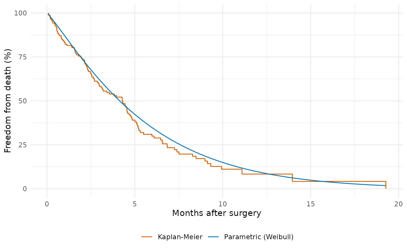
# -- Parametric survival with Kaplan-Meier overlay -----------------
if (requireNamespace("ggplot2", quietly = TRUE)) {
library(ggplot2)
# Parametric curve on a fine grid at median covariate profile
t_grid <- seq(0.05, max(dat$time), length.out = 80)
curve_df <- data.frame(
time = t_grid, age = median(dat$age), nyha = 2, shock = 0
)
curve_df$survival <- predict(fit2, newdata = curve_df,
type = "survival") * 100
# Kaplan-Meier empirical overlay
km <- survival::survfit(survival::Surv(time, status) ~ 1, data = dat)
km_df <- data.frame(time = km$time, survival = km$surv * 100)
ggplot() +
geom_step(data = km_df, aes(time, survival, colour = "Kaplan-Meier")) +
geom_line(data = curve_df, aes(time, survival,
colour = "Parametric (Weibull)")) +
scale_colour_manual(
values = c("Parametric (Weibull)" = "#0072B2",
"Kaplan-Meier" = "#D55E00")
) +
scale_y_continuous(limits = c(0, 100)) +
labs(x = "Months after surgery", y = "Freedom from death (%)",
colour = NULL) +
theme_minimal() +
theme(legend.position = "bottom")
}
 # }
# \donttest{
# -- Multiphase model (two phases) ---------------------------------
fit_mp <- hazard(
survival::Surv(time, status) ~ 1,
data = dat,
dist = "multiphase",
phases = list(
early = hzr_phase("cdf", t_half = 0.5, nu = 2, m = 0,
fixed = "shapes"),
late = hzr_phase("cdf", t_half = 5, nu = 1, m = 0,
fixed = "shapes")
),
fit = TRUE,
control = list(n_starts = 5, maxit = 1000)
)
summary(fit_mp)
#> Multiphase hazard model (2 phases)
#> observations: 180
#> predictors: 0
#> dist: multiphase
#> phase 1: early - cdf (early risk)
#> phase 2: late - cdf (late risk)
#> engine: native-r-m2
#> converged: TRUE
#> gradient: relative 3.74e-10 (SAS/C requires <= 6.06e-06; met, nlm code 1)
#> log-lik: -321.926
#> Not done in this run: none
#> evaluations: fn=26, gr=7
#> message: continued with nlm() for 1 iterations (code 1)
#>
#> Coefficients (internal scale):
#>
#> Phase: early (cdf)
#> estimate std_error z_stat p_value
#> log_mu -1.8214603 0.270271 -6.739385 1.590589e-11
#> log_t_half -0.6931472 NA NA NA
#> nu 2.0000000 NA NA NA
#> m 0.0000000 NA NA NA
#>
#> Phase: late (cdf)
#> estimate std_error z_stat p_value
#> log_mu 0.6120246 0.1098426 5.571832 2.52075e-08
#> log_t_half 1.6094379 NA NA NA
#> nu 1.0000000 NA NA NA
#> m 0.0000000 NA NA NA
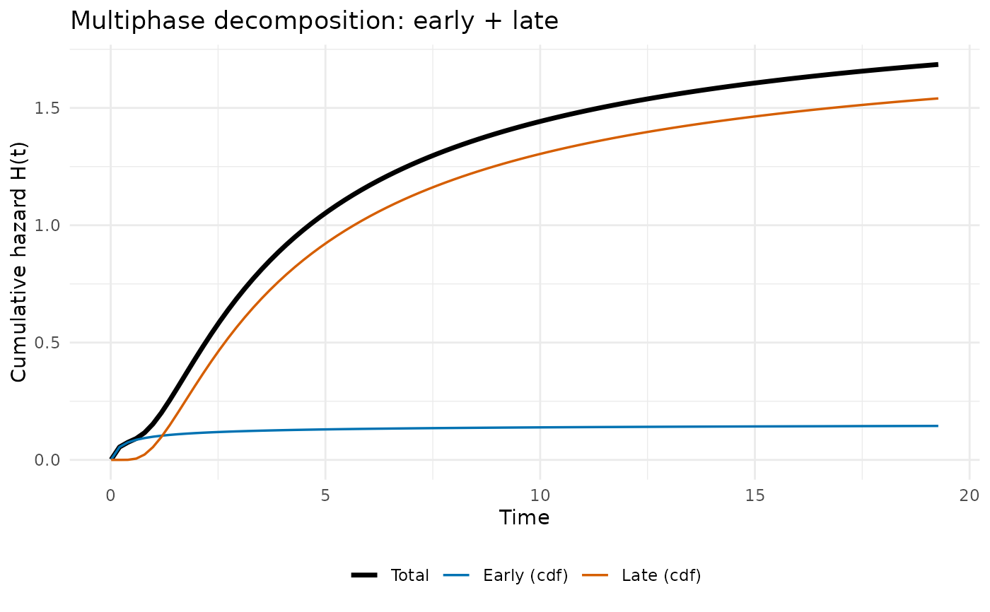
# -- Per-phase decomposed cumulative hazard ------------------------
if (requireNamespace("ggplot2", quietly = TRUE)) {
t_grid <- seq(0.01, max(dat$time), length.out = 100)
decomp <- predict(fit_mp, newdata = data.frame(time = t_grid),
type = "cumulative_hazard", decompose = TRUE)
df_long <- data.frame(
time = rep(decomp$time, 3),
cumhaz = c(decomp$total, decomp$early, decomp$late),
component = rep(c("Total", "Early (cdf)", "Late (cdf)"),
each = nrow(decomp))
)
df_long$component <- factor(df_long$component,
levels = c("Total", "Early (cdf)", "Late (cdf)"))
ggplot2::ggplot(df_long,
ggplot2::aes(x = time, y = cumhaz, colour = component,
linewidth = component)) +
ggplot2::geom_line() +
ggplot2::scale_colour_manual(values = c(
"Total" = "black", "Early (cdf)" = "#0072B2",
"Late (cdf)" = "#D55E00"
)) +
ggplot2::scale_linewidth_manual(values = c(
"Total" = 1.2, "Early (cdf)" = 0.6, "Late (cdf)" = 0.6
)) +
ggplot2::labs(
x = "Time", y = "Cumulative hazard H(t)",
colour = NULL, linewidth = NULL,
title = "Multiphase decomposition: early + late"
) +
ggplot2::theme_minimal() +
ggplot2::theme(legend.position = "bottom")
}
# }
# \donttest{
# -- Multiphase model (two phases) ---------------------------------
fit_mp <- hazard(
survival::Surv(time, status) ~ 1,
data = dat,
dist = "multiphase",
phases = list(
early = hzr_phase("cdf", t_half = 0.5, nu = 2, m = 0,
fixed = "shapes"),
late = hzr_phase("cdf", t_half = 5, nu = 1, m = 0,
fixed = "shapes")
),
fit = TRUE,
control = list(n_starts = 5, maxit = 1000)
)
summary(fit_mp)
#> Multiphase hazard model (2 phases)
#> observations: 180
#> predictors: 0
#> dist: multiphase
#> phase 1: early - cdf (early risk)
#> phase 2: late - cdf (late risk)
#> engine: native-r-m2
#> converged: TRUE
#> gradient: relative 3.74e-10 (SAS/C requires <= 6.06e-06; met, nlm code 1)
#> log-lik: -321.926
#> Not done in this run: none
#> evaluations: fn=26, gr=7
#> message: continued with nlm() for 1 iterations (code 1)
#>
#> Coefficients (internal scale):
#>
#> Phase: early (cdf)
#> estimate std_error z_stat p_value
#> log_mu -1.8214603 0.270271 -6.739385 1.590589e-11
#> log_t_half -0.6931472 NA NA NA
#> nu 2.0000000 NA NA NA
#> m 0.0000000 NA NA NA
#>
#> Phase: late (cdf)
#> estimate std_error z_stat p_value
#> log_mu 0.6120246 0.1098426 5.571832 2.52075e-08
#> log_t_half 1.6094379 NA NA NA
#> nu 1.0000000 NA NA NA
#> m 0.0000000 NA NA NA
# -- Per-phase decomposed cumulative hazard ------------------------
if (requireNamespace("ggplot2", quietly = TRUE)) {
t_grid <- seq(0.01, max(dat$time), length.out = 100)
decomp <- predict(fit_mp, newdata = data.frame(time = t_grid),
type = "cumulative_hazard", decompose = TRUE)
df_long <- data.frame(
time = rep(decomp$time, 3),
cumhaz = c(decomp$total, decomp$early, decomp$late),
component = rep(c("Total", "Early (cdf)", "Late (cdf)"),
each = nrow(decomp))
)
df_long$component <- factor(df_long$component,
levels = c("Total", "Early (cdf)", "Late (cdf)"))
ggplot2::ggplot(df_long,
ggplot2::aes(x = time, y = cumhaz, colour = component,
linewidth = component)) +
ggplot2::geom_line() +
ggplot2::scale_colour_manual(values = c(
"Total" = "black", "Early (cdf)" = "#0072B2",
"Late (cdf)" = "#D55E00"
)) +
ggplot2::scale_linewidth_manual(values = c(
"Total" = 1.2, "Early (cdf)" = 0.6, "Late (cdf)" = 0.6
)) +
ggplot2::labs(
x = "Time", y = "Cumulative hazard H(t)",
colour = NULL, linewidth = NULL,
title = "Multiphase decomposition: early + late"
) +
ggplot2::theme_minimal() +
ggplot2::theme(legend.position = "bottom")
}
 # }
# }