Predict from a hazard model object

Produces prediction outputs from a hazard object. Supports multiple prediction types including linear predictor, hazard, survival probability, and cumulative hazard.

Usage

# S3 method for class 'hazard'
predict(
  object,
  newdata = NULL,
  type = c("hazard", "linear_predictor", "survival", "cumulative_hazard"),
  decompose = FALSE,
  se.fit = FALSE,
  level = 0.95,
  conf.type = c("log-log", "logit"),
  ...
)

Arguments

object

A hazard object.

newdata

Optional matrix or data frame of predictors. For types requiring time (e.g., "survival", "cumulative_hazard"), newdata should include a time column, or time will be taken from the fitted object's data.

type

Prediction type:

"linear_predictor": Linear predictor eta = x*beta (not available for multiphase)
"hazard": Instantaneous hazard. Single-distribution models return the hazard scale exp(eta); multiphase models return the additive hazard h(t|x) = sum_j mu_j(x) phi_j'(t) and so require time values (like "survival"/"cumulative_hazard"). decompose is not supported for "hazard".
"survival": Survival probability S(t|x) = exp(-H(t|x))
"cumulative_hazard": Cumulative hazard H(t|x) at event times

decompose

Logical; if TRUE and the model is multiphase, return a data frame with per-phase cumulative hazard contributions alongside the total. Ignored for single-distribution models. Default FALSE.

se.fit

Logical; if TRUE, compute delta-method standard errors and confidence limits for each prediction. The return value becomes a data frame with columns fit, se.fit, lower, upper. Default FALSE. CLs are computed on the log-hazard / log-cumhaz scale and on the log(-log(survival)) scale so lower/upper stay inside the valid range of each prediction type; linear_predictor uses symmetric natural-scale CLs. For multiphase models, se.fit = TRUE combines with decompose = TRUE when type = "cumulative_hazard": the result is a long data frame with one row per prediction time and component (component in "total" plus each phase name) and columns fit, se.fit, lower, upper. Per-phase CLs use only that phase's parameters, so they do not sum to the total CL. The combination is not available for type = "survival" (per-phase survival is not additive).

level

Numeric confidence level in (0, 1); default 0.95. Only used when se.fit = TRUE.

SAS draws narrower bands than this by default. PROC HAZPRED takes its width from CLEVEL, whose default is 0.68268948 — documented in the macro source as "(1 sd)" — so its T_ALPHA multiplier is 1 to seven decimals (the literal is truncated) and the band is one standard error, 68.3%, not 95%. Reproducing a SAS figure at this function's default therefore yields a band about 1.96 times wider than the one being checked against, with no error and no warning on either side. Pass the SAS level explicitly to match:

predict(fit, newdata, type = "survival", se.fit = TRUE,
        level = 2 * stats::pnorm(1) - 1, conf.type = "logit")

The default is left at 0.95 deliberately: it is the right R-side default, and silently adopting SAS's would make this method disagree with every other R modelling function.

conf.type

Transform for type = "survival" confidence limits when se.fit = TRUE: "log-log" (default) builds them on log(-log S) (the survival::survfit standard); "logit" builds them on logit(1 - S), reproducing SAS HAZARD's HAZPRED survival limits. Other types are unaffected (hazard/cumulative-hazard use a log scale that already matches HAZPRED). Only used when se.fit = TRUE.

...

Unused; included for S3 compatibility.

Value

When se.fit = FALSE (default), a numeric vector of predictions. When se.fit = TRUE, a data frame with columns fit, se.fit, lower, upper (delta-method point estimate, standard error, and confidence limits at level). For multiphase type = "cumulative_hazard" with decompose = TRUE, a long data frame (time, component, fit, se.fit, lower, upper); with decompose = TRUE and se.fit = FALSE, a wide data frame of per-phase contributions.

Details

For Weibull models with survival or cumulative_hazard predictions:

Cumulative hazard: H(t|x) = (mu*t)^nu * exp(eta)
Survival: S(t|x) = exp(-H(t|x))

Time values must be positive and finite. If newdata contains a time column, it will be used; otherwise, the time vector from the fitted object is used. For models fit with time_windows, predictions for type = "linear_predictor" or "hazard" also require time values (via newdata$time or fitted-time fallback) so window-specific coefficients can be selected.

Examples

# -- Basic predictions ------------------------------------------------
set.seed(1)
fit <- hazard(time = rexp(50, 0.3), status = rep(1L, 50),
              theta = c(0.3, 1.0), dist = "weibull", fit = TRUE)
predict(fit, type = "survival")
#>  [1] 0.508448836 0.315117497 0.909632142 0.913801355 0.704022509 0.034429522
#>  [7] 0.297904379 0.635876619 0.407732732 0.908685617 0.245861859 0.504733067
#> [13] 0.295096862 0.003729697 0.364948062 0.373066533 0.134498594 0.565324696
#> [19] 0.772692686 0.605268524 0.070992893 0.572924045 0.803140735 0.619329758
#> [25] 0.937239852 0.968075472 0.611315229 0.007471798 0.318195648 0.389681823
#> [31] 0.232969073 0.981596565 0.781843506 0.267479469 0.868327070 0.378412625
#> [37] 0.797695039 0.524953194 0.510431884 0.845615583 0.354514703 0.376046945
#> [43] 0.276615587 0.289749395 0.626388405 0.798022001 0.276332062 0.390676459
#> [49] 0.652266897 0.113525051
predict(fit, newdata = data.frame(time = c(1, 2, 5)),
        type = "cumulative_hazard")
#> [1] 0.2244716 0.5138491 1.5356737

# -- Patient-specific survival curves ---------------------------------
set.seed(1001)
n   <- 180
dat <- data.frame(
  time   = rexp(n, rate = 0.35) + 0.05,
  status = rbinom(n, size = 1, prob = 0.6),
  age    = rnorm(n, mean = 62, sd = 11),
  nyha   = sample(1:4, n, replace = TRUE),
  shock  = rbinom(n, size = 1, prob = 0.18)
)
fit2 <- hazard(
  survival::Surv(time, status) ~ age + nyha + shock,
  data  = dat,
  theta = c(mu = 0.25, nu = 1.10, beta1 = 0, beta2 = 0, beta3 = 0),
  dist  = "weibull", fit = TRUE
)

new_patients <- data.frame(
  time = c(0.5, 1.5, 3.0),
  age  = c(50, 65, 75),
  nyha = c(1, 3, 4),
  shock = c(0, 0, 1)
)
# Compute predictions from the clean covariate frame before adding columns
surv   <- predict(fit2, newdata = new_patients, type = "survival")
cumhaz <- predict(fit2, newdata = new_patients, type = "cumulative_hazard")
new_patients$survival          <- surv
new_patients$cumulative_hazard <- cumhaz
new_patients
#>   time age nyha shock  survival cumulative_hazard
#> 1  0.5  50    1     0 0.9494097        0.05191482
#> 2  1.5  65    3     0 0.7743185        0.25577202
#> 3  3.0  75    4     1 0.5046535        0.68388317

# \donttest{
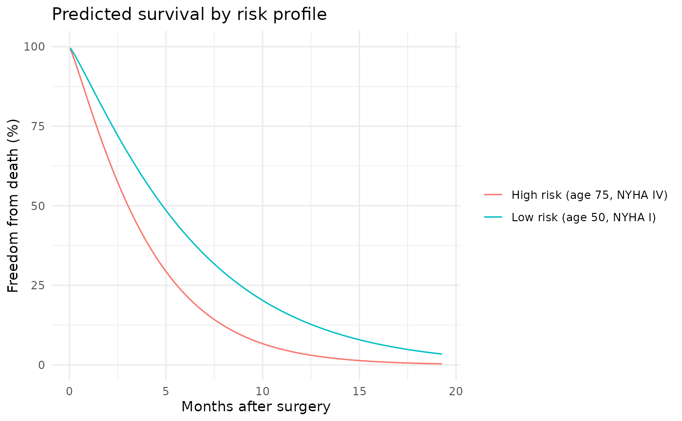
# -- Grouped survival curves ---------------------------------------
if (requireNamespace("ggplot2", quietly = TRUE)) {
  library(ggplot2)

  t_grid <- seq(0.05, max(dat$time), length.out = 80)
  profiles <- data.frame(
    label = c("Low risk (age 50, NYHA I)",
              "High risk (age 75, NYHA IV)"),
    age   = c(50, 75),
    nyha  = c(1, 4),
    shock = c(0, 1)
  )

  curve_list <- lapply(seq_len(nrow(profiles)), function(i) {
    nd <- data.frame(
      time  = t_grid,
      age   = profiles$age[i],
      nyha  = profiles$nyha[i],
      shock = profiles$shock[i]
    )
    nd$survival <- predict(fit2, newdata = nd, type = "survival") * 100
    nd$profile  <- profiles$label[i]
    nd
  })
  curve_df <- do.call(rbind, curve_list)

  ggplot(curve_df, aes(time, survival, colour = profile)) +
    geom_line() +
    scale_y_continuous(limits = c(0, 100)) +
    labs(x = "Months after surgery",
         y = "Freedom from death (%)",
         title = "Predicted survival by risk profile",
         colour = NULL) +
    theme_minimal()
}

# }

# \donttest{
# -- Multiphase predictions with decomposition --------------------
set.seed(42)
n   <- 200
dat <- data.frame(
  time   = rexp(n, rate = 0.25) + 0.01,
  status = rbinom(n, size = 1, prob = 0.65)
)
fit_mp <- hazard(
  survival::Surv(time, status) ~ 1,
  data   = dat,
  dist   = "multiphase",
  phases = list(
    early = hzr_phase("cdf", t_half = 0.5, nu = 2, m = 0,
                       fixed = "shapes"),
    late  = hzr_phase("cdf", t_half = 5,   nu = 1, m = 0,
                       fixed = "shapes")
  ),
  fit     = TRUE,
  control = list(n_starts = 5, maxit = 1000)
)

t_grid <- seq(0.01, max(dat$time) * 0.9, length.out = 100)
nd     <- data.frame(time = t_grid)

# Overall survival
predict(fit_mp, newdata = nd, type = "survival")
#> early.log_mu early.log_mu early.log_mu early.log_mu early.log_mu early.log_mu 
#>    0.9991035    0.9506784    0.9308151    0.8914460    0.8319957    0.7661075 
#> early.log_mu early.log_mu early.log_mu early.log_mu early.log_mu early.log_mu 
#>    0.7030006    0.6464725    0.5973331    0.5551218    0.5189604    0.4879203 
#> early.log_mu early.log_mu early.log_mu early.log_mu early.log_mu early.log_mu 
#>    0.4611599    0.4379620    0.4177325    0.3999854    0.3843245    0.3704267 
#> early.log_mu early.log_mu early.log_mu early.log_mu early.log_mu early.log_mu 
#>    0.3580277    0.3469105    0.3368956    0.3278342    0.3196018    0.3120940 
#> early.log_mu early.log_mu early.log_mu early.log_mu early.log_mu early.log_mu 
#>    0.3052225    0.2989124    0.2930997    0.2877295    0.2827546    0.2781339 
#> early.log_mu early.log_mu early.log_mu early.log_mu early.log_mu early.log_mu 
#>    0.2738318    0.2698173    0.2660630    0.2625450    0.2592421    0.2561355 
#> early.log_mu early.log_mu early.log_mu early.log_mu early.log_mu early.log_mu 
#>    0.2532086    0.2504463    0.2478356    0.2453643    0.2430218    0.2407985 
#> early.log_mu early.log_mu early.log_mu early.log_mu early.log_mu early.log_mu 
#>    0.2386855    0.2366750    0.2347598    0.2329333    0.2311896    0.2295232 
#> early.log_mu early.log_mu early.log_mu early.log_mu early.log_mu early.log_mu 
#>    0.2279292    0.2264030    0.2249404    0.2235376    0.2221909    0.2208972 
#> early.log_mu early.log_mu early.log_mu early.log_mu early.log_mu early.log_mu 
#>    0.2196533    0.2184565    0.2173041    0.2161938    0.2151234    0.2140906 
#> early.log_mu early.log_mu early.log_mu early.log_mu early.log_mu early.log_mu 
#>    0.2130936    0.2121306    0.2111998    0.2102997    0.2094289    0.2085858 
#> early.log_mu early.log_mu early.log_mu early.log_mu early.log_mu early.log_mu 
#>    0.2077692    0.2069779    0.2062107    0.2054665    0.2047444    0.2040434 
#> early.log_mu early.log_mu early.log_mu early.log_mu early.log_mu early.log_mu 
#>    0.2033625    0.2027009    0.2020578    0.2014325    0.2008241    0.2002321 
#> early.log_mu early.log_mu early.log_mu early.log_mu early.log_mu early.log_mu 
#>    0.1996558    0.1990946    0.1985478    0.1980150    0.1974957    0.1969892 
#> early.log_mu early.log_mu early.log_mu early.log_mu early.log_mu early.log_mu 
#>    0.1964951    0.1960131    0.1955426    0.1950833    0.1946347    0.1941965 
#> early.log_mu early.log_mu early.log_mu early.log_mu early.log_mu early.log_mu 
#>    0.1937683    0.1933498    0.1929407    0.1925406    0.1921493    0.1917665 
#> early.log_mu early.log_mu early.log_mu early.log_mu 
#>    0.1913919    0.1910252    0.1906662    0.1903146 

# Per-phase decomposed cumulative hazard
decomp <- predict(fit_mp, newdata = nd,
                  type = "cumulative_hazard", decompose = TRUE)
head(decomp)
#>        time        total        early          late
#> 1 0.0100000 0.0008968883 0.0008968883 5.301131e-151
#> 2 0.3177112 0.0505794621 0.0505477015  3.176054e-05
#> 3 0.6254224 0.0716946604 0.0648908394  6.803821e-03
#> 4 0.9331336 0.1149103629 0.0726084041  4.230196e-02
#> 5 1.2408448 0.1839280141 0.0776698937  1.062581e-01
#> 6 1.5485560 0.2664327951 0.0813370883  1.850957e-01
# }

Usage

Arguments

Value

Details

See also

Examples