Complete Clinical Analysis Walkthrough • TemporalHazard

The previous vignettes covered each piece of the analytical workflow in isolation: how to fit a model, how to predict from it, how to validate it. This vignette runs all of those pieces together on a single dataset, in the order you’d actually run them in a real clinical analysis. The point isn’t to introduce new functions; it’s to show how the pieces chain into a disciplined sequence that turns raw covariates into a fitted, validated, defensible hazard model.

The sequence mirrors the one in the original SAS HAZARD system, which codified what cardiothoracic-surgery biostatisticians had been doing informally for decades:

Nonparametric baseline: Kaplan-Meier life table to see what the data is saying before any model intervenes.
Shape fitting: start with a single-distribution Weibull, build up to a multiphase decomposition when the KM curve demands it.
Variable screening: univariable association tests and calibration plots to decide which covariates enter the model and in what functional form.
Multivariable model: covariates layered onto a hazard shape you already trust.
Prediction: patient-specific risk profiles for clinical reporting and decision support.
Validation: decile-of-risk calibration to verify the model is honest across the risk spectrum, not just on average.

This corresponds to the SAS programs ac.* → hz.* → lg.* → hm.* → hp.* → hs.*. If you’re familiar with the SAS workflow, the section structure should feel familiar; if not, treat this as the canonical analytical sequence to follow on any new dataset.

We use the AVC dataset (310 patients, atrioventricular canal repair) which has rich covariates and two identifiable hazard phases. That is fewer phases than the 3-phase CABG example you’ve seen in other vignettes, but AVC has the covariate complexity needed to exercise the screening, multivariable-fit, and validation steps.

1 Data preparation

Load the package and the AVC dataset, drop incomplete rows so the design matrix is rectangular for the multivariable fits to come, and inspect the resulting column types and ranges. The na.omit() step is conservative (losing rows is a real cost), but for a walkthrough we want every later fit to use the same patient set so the comparisons are apples-to-apples.

library(TemporalHazard)
if (has_ggplot2) library(ggplot2)

data(avc)
avc <- na.omit(avc)
str(avc)
#> 'data.frame':    305 obs. of  11 variables:
#>  $ study   : chr  "001C" "002C" "004C" "005C" ...
#>  $ status  : int  3 3 1 2 2 3 1 1 3 3 ...
#>  $ inc_surg: int  4 3 2 3 1 2 3 2 3 3 ...
#>  $ opmos   : num  9.46 34.07 51.58 55 60.65 ...
#>  $ age     : num  69.2 53.7 286.1 154.6 48.4 ...
#>  $ mal     : int  0 0 0 1 0 0 0 0 0 0 ...
#>  $ com_iv  : int  1 1 1 1 1 1 1 1 1 1 ...
#>  $ orifice : int  0 0 0 0 0 0 0 0 0 0 ...
#>  $ dead    : int  1 1 0 0 0 0 0 0 0 1 ...
#>  $ int_dead: num  0.0534 0.3778 91.5337 111.608 106.8112 ...
#>  $ op_age  : num  654 1828 14759 8505 2933 ...
#>  - attr(*, "na.action")= 'omit' Named int [1:5] 12 90 138 144 146
#>   ..- attr(*, "names")= chr [1:5] "12" "90" "138" "144" ...

The AVC dataset contains 305 patients after removing incomplete cases. Key covariates include age at repair (age, in months), NYHA functional class (status), presence of malalignment (mal), and interventricular communication (com_iv).

2 Step 1: Nonparametric baseline

Before fitting any parametric model, establish the empirical survival curve using the Kaplan-Meier estimator. This is the benchmark against which all parametric fits will be compared.

hzr_kaplan() wraps survival::survfit() and adds logit-transformed exact confidence limits that respect the [0, 1] boundary and are more accurate in the tails than the default Greenwood intervals. This matches the SAS kaplan.sas macro output structure.

km <- hzr_kaplan(time = avc$int_dead, status = avc$dead)
head(km)
#> Kaplan-Meier estimate with logit confidence limits
#> Events: 18  | Time points: 6 
#> Survival range: 0.941 to 0.9836 
#> RMST at last event: 0.0472 
#> 
#>         time n_risk n_event n_censor survival std_err cl_lower cl_upper cumhaz
#>  0.001368954    305       5        0   0.9836  0.0073   0.9612   0.9932 0.0165
#>  0.002737907    300       2        0   0.9770  0.0086   0.9527   0.9890 0.0232
#>  0.008213721    298       2        0   0.9705  0.0097   0.9443   0.9846 0.0300
#>  0.016427440    296       5        0   0.9541  0.0120   0.9240   0.9726 0.0470
#>  0.032854880    291       3        0   0.9443  0.0131   0.9122   0.9651 0.0574
#>  0.049282330    288       1        0   0.9410  0.0135   0.9083   0.9625 0.0608
#>   hazard density   life
#>  12.0744 11.9752 0.0014
#>   4.8862  4.7901 0.0027
#>   1.2298  1.1975 0.0081
#>   2.0741  1.9959 0.0160
#>   0.6308  0.5988 0.0317
#>   0.2117  0.1996 0.0472

The returned data frame is the life table: one row per event time with n_risk, n_event, survival, logit-transformed 95% CLs (cl_lower / cl_upper), and a KM-based cumulative hazard (-log(survival); use hzr_nelson() if you need the Nelson-Aalen estimator instead). The plot uses the survival column for the step curve and the two confidence limits for the band:

km_df <- data.frame(
  time     = km$time,
  survival = km$survival * 100,
  lower    = km$cl_lower * 100,
  upper    = km$cl_upper * 100
)

ggplot(km_df, aes(time, survival)) +
  geom_step(colour = "#D55E00", linewidth = 0.8) +
  geom_ribbon(aes(ymin = lower, ymax = upper),
              stat = "identity", alpha = 0.15, fill = "#D55E00") +
  labs(x = "Months after AVC repair", y = "Survival (%)") +
  coord_cartesian(ylim = c(0, 100)) +
  theme_minimal()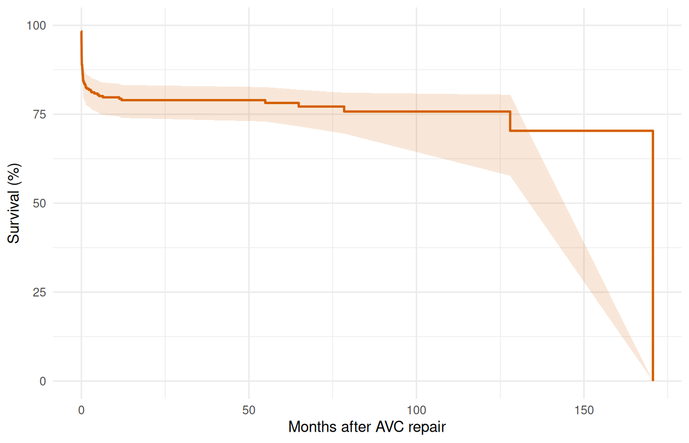

Figure 1: Kaplan-Meier survival estimate for AVC patients (n = 305)

The KM curve shows a sharp early drop (operative mortality) followed by a roughly constant attrition rate. This two-phase pattern suggests an early CDF phase plus a constant phase, with no obvious late rising hazard.

3 Step 2: Shape fitting (simple to complex)

3.1 2a. Single-phase Weibull

The discipline here is to start with the simplest parametric model and earn any added complexity. A single-distribution Weibull intercept-only fit gives us a smooth two-parameter curve to compare against the KM baseline. If the Weibull tracks the KM step function reasonably well, we may be done; if it can’t, the gap tells us exactly where a richer model needs to go.

fit_weib <- hazard(
  survival::Surv(int_dead, dead) ~ 1,
  data  = avc,
  dist  = "weibull",
  theta = c(mu = 0.05, nu = 0.5),
  fit   = TRUE
)
summary(fit_weib)
#> hazard model summary
#>   observations: 305 
#>   predictors:   0 
#>   dist:         weibull 
#>   engine:       native-r-m2 
#>   converged:    TRUE 
#>   gradient:     relative 2.99e-06 (SAS/C requires <= 6.06e-06; met, nlm code 1)
#>   log-lik:      -234.774 
#>   Not done in this run: none
#>   evaluations: fn=34, gr=9
#>   message:      continued with nlm() for 4 iterations (code 1) 
#> 
#> Coefficients:
#>        estimate    std_error   z_stat      p_value
#> mu 3.509006e-05 3.463678e-05 1.013087 3.110187e-01
#> nu 2.043723e-01 2.332197e-02 8.763081 1.899849e-18

The Weibull forces a monotone hazard shape. Let’s overlay it on the Kaplan-Meier to see where it fits well and where it doesn’t.

t_grid <- seq(0.01, max(avc$int_dead) * 0.9, length.out = 200)
surv_weib <- predict(fit_weib,
                     newdata = data.frame(time = t_grid),
                     type = "survival") * 100

ggplot() +
  geom_step(data = km_df, aes(time, survival),
            colour = "#D55E00", linewidth = 0.6) +
  geom_line(data = data.frame(time = t_grid, survival = surv_weib),
            aes(time, survival), colour = "#0072B2", linewidth = 0.8) +
  labs(x = "Months after AVC repair", y = "Survival (%)") +
  coord_cartesian(ylim = c(0, 100)) +
  theme_minimal()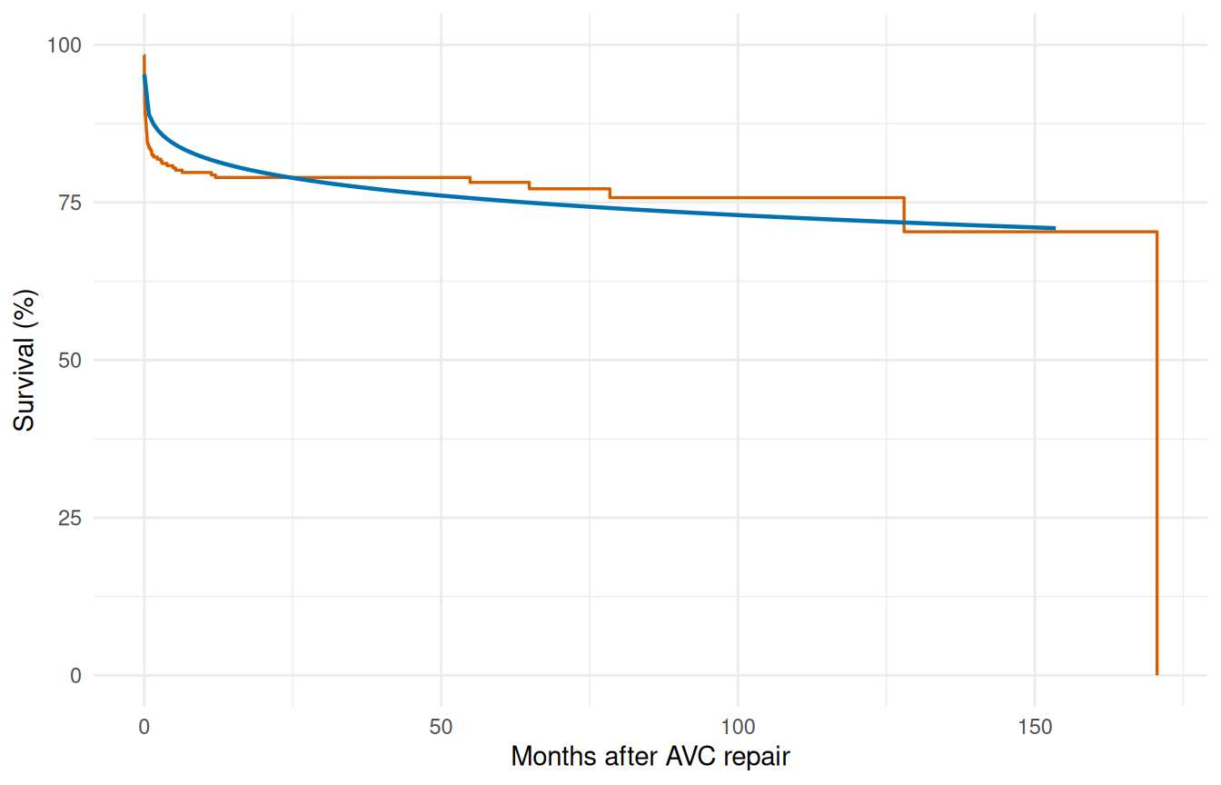

Figure 2: Single Weibull vs. Kaplan-Meier

The single Weibull typically misses the sharp early drop; it compromises between the early and late time frames.

3.2 2b. Two-phase model (early CDF + constant)

The KM curve drops steeply in the first few months (operative mortality) and then settles into a roughly linear decline. The Weibull tried to capture both with one shape and ended up compromising. Splitting the hazard into two phases lets each mechanism have its own parameterization: a "cdf" early phase that saturates as operative risk resolves, plus a "constant" phase that carries the steady background attrition. Two phases is what AVC actually needs; CABG with longer follow-up would need a third late-rising phase to handle graft deterioration, but the AVC follow-up window doesn’t extend far enough to identify one.

fit_mp <- hazard(
  survival::Surv(int_dead, dead) ~ 1,
  data   = avc,
  dist   = "multiphase",
  phases = list(
    early    = hzr_phase("cdf", t_half = 0.5, nu = 1, m = 1,
                          fixed = "shapes"),
    constant = hzr_phase("constant")
  ),
  fit     = TRUE,
  control = list(n_starts = 5, maxit = 1000)
)
summary(fit_mp)
#> Multiphase hazard model (2 phases)
#>   observations: 305 
#>   predictors:   0 
#>   dist:         multiphase 
#>   phase 1:      early - cdf (early risk)
#>   phase 2:      constant - constant (flat rate)
#>   engine:       native-r-m2 
#>   converged:    TRUE 
#>   gradient:     relative 1.27e-09 (SAS/C requires <= 6.06e-06; met, nlm code 1)
#>   log-lik:      -228.029 
#>   Not done in this run: none
#>   evaluations: fn=26, gr=3
#>   message:      continued with nlm() for 1 iterations (code 1) 
#> 
#> Coefficients (internal scale):
#> 
#>   Phase: early (cdf)
#>                estimate std_error    z_stat     p_value
#>   log_mu     -1.4132735 0.1290435 -10.95192 6.50568e-28
#>   log_t_half -0.6931472        NA        NA          NA
#>   nu          1.0000000        NA        NA          NA
#>   m           1.0000000        NA        NA          NA
#> 
#>   Phase: constant (constant)
#>           estimate std_error    z_stat      p_value
#>   log_mu -7.609476 0.4495826 -16.92564 2.911456e-64

Note the use of fixed = "shapes". We fix the temporal shape parameters and only estimate the scale (log_mu) for each phase. This matches the standard HAZARD workflow: shapes are set from clinical knowledge or preliminary exploration, then scales and covariates are estimated.

surv_mp <- predict(fit_mp,
                   newdata = data.frame(time = t_grid),
                   type = "survival") * 100

ggplot() +
  geom_step(data = km_df, aes(time, survival),
            colour = "#D55E00", linewidth = 0.6) +
  geom_line(data = data.frame(time = t_grid, survival = surv_mp),
            aes(time, survival), colour = "#0072B2", linewidth = 0.8) +
  labs(x = "Months after AVC repair", y = "Survival (%)") +
  coord_cartesian(ylim = c(0, 100)) +
  theme_minimal()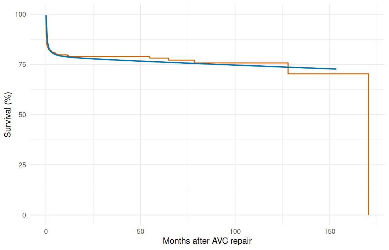

Figure 3: Two-phase parametric model vs. Kaplan-Meier

3.3 2c. Decomposed hazard

The overlay plot shows the total fit tracks KM well, but it doesn’t show whether each phase is doing the job we asked of it. Decomposing the cumulative hazard into per-phase contributions is the diagnostic that answers that question: the early phase should account for most of the steep early drop, the constant phase should carry the rest, and neither phase should be doing implausible work in the wrong time window.

decomp <- predict(fit_mp,
                  newdata = data.frame(time = t_grid),
                  type = "cumulative_hazard",
                  decompose = TRUE)

decomp_df <- data.frame(
  time  = t_grid,
  total = decomp[, "total"],
  early = decomp[, "early"],
  const = decomp[, "constant"]
)

ggplot(decomp_df, aes(x = time)) +
  geom_line(aes(y = total), linewidth = 0.9, colour = "black") +
  geom_line(aes(y = early), linewidth = 0.7, colour = "#E69F00",
            linetype = "dashed") +
  geom_line(aes(y = const), linewidth = 0.7, colour = "#56B4E9",
            linetype = "dashed") +
  labs(x = "Months after AVC repair", y = "Cumulative hazard") +
  theme_minimal()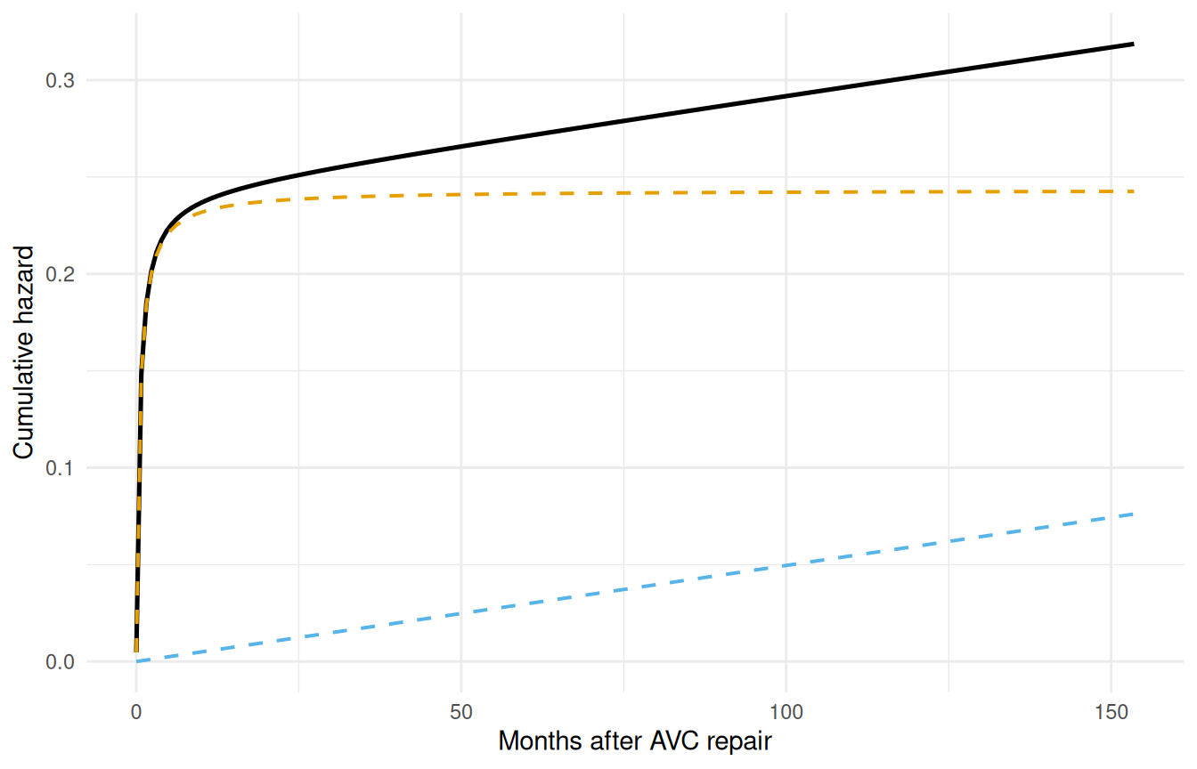

Figure 4: Phase decomposition of cumulative hazard

The early phase contributes most of its risk in the first few months, then levels off. The constant phase accumulates linearly over time.

4 Step 3: Variable screening

Before entering covariates into the hazard model, screen them for association with the outcome. This step corresponds to the lg.* programs in the SAS workflow.

4.1 3a. Univariable logistic screening

The cheapest screening tool we have is a univariable logistic regression of the event indicator on each covariate. It throws away the time-to-event structure but it answers a binary question quickly: does this covariate have any association with mortality at all? Covariates whose univariable p-value is huge can be deprioritized, but not discarded outright, because adjusting for other covariates can reveal an association the univariable test misses. Covariates with small univariable p-values deserve closer functional-form inspection before they enter the formula.

covariates <- c("age", "status", "mal", "com_iv", "orifice",
                "inc_surg", "opmos")

screen_results <- data.frame(
  variable = covariates,
  coef     = numeric(length(covariates)),
  p_value  = numeric(length(covariates))
)

for (i in seq_along(covariates)) {
  v <- covariates[i]
  fml <- as.formula(paste("dead ~", v))
  lg <- glm(fml, data = avc, family = binomial)
  s <- summary(lg)$coefficients
  if (nrow(s) >= 2) {
    screen_results$coef[i] <- s[2, 1]
    screen_results$p_value[i] <- s[2, 4]
  }
}

screen_results <- screen_results[order(screen_results$p_value), ]
screen_results$significant <- ifelse(screen_results$p_value < 0.05,
                                      "*", "")
screen_results
#>   variable         coef      p_value significant
#> 2   status  0.965232352 2.538365e-08           *
#> 4   com_iv  1.413423027 4.916970e-06           *
#> 3      mal  1.027084963 6.478986e-04           *
#> 1      age -0.004914258 1.683468e-03           *
#> 5  orifice  1.635755221 3.440489e-03           *
#> 6 inc_surg  0.293339962 1.144172e-02           *
#> 7    opmos  0.001458721 6.552347e-01

4.2 3b. Functional form assessment

For continuous covariates that appear significant, examine whether the relationship with outcome is monotone on the logit scale. hzr_calibrate() implements the SAS logit.sas / logitgr.sas macros: bin the continuous covariate into quantile groups, compute the observed event rate per bin, and transform it to the logit scale.

cal_age <- hzr_calibrate(x = avc$age, event = avc$dead,
                          groups = 10, link = "logit")
cal_age
#> Variable calibration (logit link, 10 groups)
#> 
#>  group  n events    mean     min     max  prob link_value
#>      1 30     11   3.519   1.051   5.388 0.367     -0.547
#>      2 31     11   8.665   5.421  11.532 0.355     -0.598
#>      3 30     13  15.194  11.631  18.497 0.433     -0.268
#>      4 31     11  23.077  18.990  27.828 0.355     -0.598
#>      5 30      7  43.544  28.124  57.167 0.233     -1.190
#>      6 31      3  72.066  59.730  86.408 0.097     -2.234
#>      7 30      2 101.154  86.507 117.522 0.067     -2.639
#>      8 31      3 162.739 121.169 203.733 0.097     -2.234
#>      9 30      4 247.051 205.343 297.140 0.133     -1.872
#>     10 31      3 530.623 324.573 790.981 0.097     -2.234

Plot the logit-transformed event rate against the bin centre (mean column). A straight line means the covariate can enter the model untransformed; monotone-but-curved shapes suggest a log or square-root transform; U-shapes call for a quadratic term.

ggplot(cal_age, aes(mean, link_value)) +
  geom_point(size = 3, colour = "#0072B2") +
  geom_line(colour = "#0072B2", alpha = 0.4) +
  geom_smooth(method = "lm", formula = y ~ x, se = FALSE,
              colour = "#D55E00", linetype = "dashed") +
  labs(x = "Age at repair (months, decile midpoint)",
       y = "logit(P(death))") +
  theme_minimal()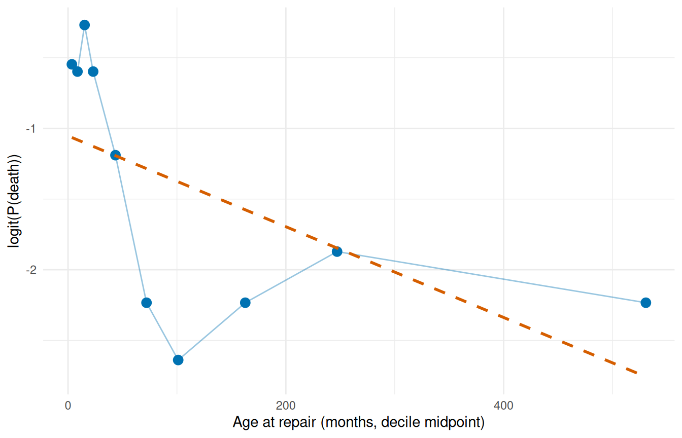

Figure 5: Decile calibration: age vs. logit(P(death))

The blue points are the observed decile logits; the dashed orange line is a linear reference. Deviations from linearity flag where a transform is warranted.

5 Step 4: Multivariable model

5.1 4a. Manual specification

We’ve already established the two-phase shape and screened the covariates; the multivariable model is the synthesis. Drop the covariates that passed screening onto the right-hand side of the formula and refit. The shape parameters stay fixed (we’ve earned that decision from §2); the optimizer estimates the two phase scales and one coefficient per covariate, jointly. This is the working model you’d report from this analysis.

fit_mv <- hazard(
  survival::Surv(int_dead, dead) ~ age + status + mal + com_iv,
  data   = avc,
  dist   = "multiphase",
  phases = list(
    early    = hzr_phase("cdf", t_half = 0.5, nu = 1, m = 1,
                          fixed = "shapes"),
    constant = hzr_phase("constant")
  ),
  fit     = TRUE,
  control = list(n_starts = 5, maxit = 1000)
)
#> Warning in .hzr_safe_solve(hess_result): Hessian is ill-conditioned (rcond =
#> 2.05e-13); standard errors may be unreliable
#> Warning in .hzr_safe_solve(hess_result): Hessian is ill-conditioned (rcond =
#> 1.17e-14); standard errors may be unreliable
#> Warning in .hzr_safe_solve(hess_result): Hessian is ill-conditioned (rcond =
#> 1.59e-11); standard errors may be unreliable
#> Warning in .hzr_safe_solve(hess_result): Hessian is ill-conditioned (rcond =
#> 1.4e-13); standard errors may be unreliable
#> Warning in .hzr_safe_solve(hess_result): Hessian is ill-conditioned (rcond =
#> 1.32e-12); standard errors may be unreliable
#> Warning in .hzr_safe_solve(H_unc): Hessian is ill-conditioned (rcond =
#> 8.64e-15); standard errors may be unreliable
summary(fit_mv)
#> Multiphase hazard model (2 phases)
#>   observations: 305 
#>   predictors:   4 
#>   dist:         multiphase 
#>   phase 1:      early - cdf (early risk)
#>   phase 2:      constant - constant (flat rate)
#>   engine:       native-r-m2 
#>   converged:    TRUE 
#>   gradient:     relative 2.17e-06 (SAS/C requires <= 6.06e-06; met, nlm code 1)
#>   log-lik:      -189.702 
#>   Note: Hessian ill-conditioned (rcond = 8.64e-15); standard errors may be unreliable.
#>   Not done in this run: none
#>   evaluations: fn=10, gr=1
#>   message:      continued with nlm() for 139 iterations (code 1) 
#> 
#> Coefficients (internal scale):
#> 
#>   Phase: early (cdf)
#>                  estimate   std_error    z_stat      p_value
#>   log_mu     -3.662542611 0.563739726 -6.496868 8.200933e-11
#>   log_t_half -0.693147181          NA        NA           NA
#>   nu          1.000000000          NA        NA           NA
#>   m           1.000000000          NA        NA           NA
#>   age        -0.002761438 0.001880896 -1.468150 1.420634e-01
#>   status      0.617748642 0.152523571  4.050185 5.117721e-05
#>   mal         0.486986741 0.271636473  1.792788 7.300675e-02
#>   com_iv      1.220199927 0.401483273  3.039230 2.371839e-03
#> 
#>   Phase: constant (constant)
#>               estimate    std_error       z_stat      p_value
#>   log_mu  -9.382415139 1.320326e+00 -7.106135447 1.193373e-12
#>   age     -0.001650775 2.498765e-03 -0.660636410 5.088455e-01
#>   status   1.068010078 4.075660e-01  2.620459314 8.781141e-03
#>   mal      0.583277928 1.140547e+00  0.511402043 6.090696e-01
#>   com_iv -20.367312072 1.395749e+04 -0.001459239 9.988357e-01

The coefficient table shows phase-specific covariate effects. A positive coefficient means higher hazard (worse prognosis). Interpretation: covariates scale the phase-specific hazard multiplicatively via exp(x * beta).

5.2 4b. Automated stepwise selection

The manual approach works when screening has already narrowed the candidate pool, but with a larger pool it helps to let the model choose. hzr_stepwise() runs forward, backward, or two-way selection against an existing hazard fit, scoring candidates with the score statistic, Wald p-values or delta-AIC. Defaults match SAS PROC HAZARD (SLENTRY = 0.30, SLSTAY = 0.20).

We start from a baseline with no covariates, offer the same screened candidate pool, and let the algorithm decide. For multiphase models the scope is a named list of one-sided formulas keyed by phase, so each phase can advertise its own candidate set; stepping operates per (variable, phase) pair, letting a covariate enter one phase and not another. Single-distribution models accept either a flat one-sided formula or a character vector of names.

hzr_stepwise() defaults to criterion = "score", which reproduces SAS’s SELECTION Q statistic by testing each candidate at the current estimates without a per-candidate refit. Here we pass criterion = "wald" deliberately, so the $steps table below reports the refit-based Wald p-values.

base_mp <- hazard(
  survival::Surv(int_dead, dead) ~ 1,
  data   = avc,
  dist   = "multiphase",
  phases = list(
    early    = hzr_phase("cdf", t_half = 0.5, nu = 1, m = 1,
                          fixed = "shapes"),
    constant = hzr_phase("constant")
  ),
  fit     = TRUE,
  control = list(n_starts = 3, maxit = 500)
)

fit_step <- hzr_stepwise(
  base_mp,
  scope     = list(
    early    = ~ age + status + mal + com_iv,
    constant = ~ age + status + mal + com_iv
  ),
  data      = avc,
  direction = "both",
  criterion = "wald",
  trace     = FALSE,
  control   = list(n_starts = 2, maxit = 500)
)
#> Warning in .hzr_safe_solve(hess_result): Hessian is ill-conditioned (rcond =
#> 7.19e-10); standard errors may be unreliable
#> Warning in .hzr_safe_solve(hess_result): Hessian is ill-conditioned (rcond =
#> 3.32e-09); standard errors may be unreliable
#> Warning in .hzr_safe_solve(H_unc): Hessian is ill-conditioned (rcond =
#> 5.76e-11); standard errors may be unreliable
#> Warning in .hzr_safe_solve(hess_result): Hessian contains non-finite entries;
#> standard errors unavailable
#> Warning in .hzr_safe_solve(hess_result): Hessian is ill-conditioned (rcond =
#> 1.36e-14); standard errors may be unreliable
#> Warning in .hzr_safe_solve(hess_result): Hessian is ill-conditioned (rcond =
#> 5.18e-12); standard errors may be unreliable
#> Warning in .hzr_safe_solve(hess_result): Hessian is ill-conditioned (rcond =
#> 1.45e-10); standard errors may be unreliable
#> Warning in .hzr_safe_solve(H_unc): Hessian is ill-conditioned (rcond =
#> 4.78e-12); standard errors may be unreliable
#> Warning in .hzr_safe_solve(hess_result): Hessian is ill-conditioned (rcond =
#> 0); standard errors may be unreliable
#> Warning in .hzr_safe_solve(hess_result): Hessian not invertible; standard
#> errors unavailable
#> Warning in .hzr_safe_solve(hess_result): Hessian is ill-conditioned (rcond =
#> 2.65e-11); standard errors may be unreliable
#> Warning in .hzr_safe_solve(hess_result): Hessian is ill-conditioned (rcond =
#> 6.95e-11); standard errors may be unreliable
#> Warning in .hzr_safe_solve(H_unc): Hessian is ill-conditioned (rcond =
#> 2.13e-11); standard errors may be unreliable
#> Warning in .hzr_safe_solve(hess_result): Hessian is ill-conditioned (rcond =
#> 1.05e-10); standard errors may be unreliable
#> Warning in .hzr_safe_solve(hess_result): Hessian is not positive-definite at
#> the optimum; standard errors may be unreliable
#> Warning in .hzr_safe_solve(hess_result): Non-positive variance estimates; the
#> optimum may not be a proper maximum
#> Warning in .hzr_safe_solve(hess_result): Hessian is ill-conditioned (rcond =
#> 4.88e-11); standard errors may be unreliable
#> Warning in .hzr_safe_solve(hess_result): Hessian is ill-conditioned (rcond =
#> 5.31e-13); standard errors may be unreliable
#> Warning in .hzr_safe_solve(H_unc): Hessian is ill-conditioned (rcond =
#> 4.34e-13); standard errors may be unreliable
#> Warning in .hzr_safe_solve(hess_result): Hessian is ill-conditioned (rcond =
#> 4.41e-19); standard errors may be unreliable
#> Warning in .hzr_safe_solve(hess_result): Hessian is ill-conditioned (rcond =
#> 4.98e-12); standard errors may be unreliable
#> Warning in .hzr_safe_solve(H_unc): Hessian is ill-conditioned (rcond =
#> 4.33e-19); standard errors may be unreliable
fit_step
#> Stepwise selection (direction = both, criterion = wald, slentry = 0.30, slstay = 0.20)
#> 
#> Step 1: ENTER  status  into  early   (p = 0.000)
#> Step 2: ENTER  com_iv  into  early   (p = 0.000)
#> Step 3: ENTER  status  into  constant   (p = 0.065)
#> Step 4: ENTER  mal  into  early   (p = 0.109)
#> Step 5: ENTER  age  into  early   (p = 0.117)
#> (no further action after 5 steps)
#> 
#> Final model: 5 covariates, logLik = -192.10, AIC = 398.21

The $steps table records every accepted action with its Wald statistic and p-value:

fit_step$steps[, c("step_num", "action", "variable", "phase",
                   "p_value", "aic")]
#>   step_num action variable    phase      p_value      aic
#> 1        1  enter   status    early 1.967175e-09 424.9675
#> 2        2  enter   com_iv    early 1.260360e-05 401.5605
#> 3        3  enter   status constant 6.500216e-02 400.3834
#> 4        4  enter      mal    early 1.094162e-01 399.8823
#> 5        5  enter      age    early 1.174822e-01 398.2062

The final model is the fit at the top of the object, reachable through the usual hazard accessors. AIC counts only the estimated parameters. Both models hold the early phase’s three shape parameters fixed (fixed = "shapes"), and fit$fit$fixed_mask flags them, so we leave them out of the count, as the Final model line of fit_step does:

logLik_manual <- fit_mv$fit$objective
logLik_step   <- fit_step$fit$objective
n_free <- function(fit) sum(!fit$fit$fixed_mask)
c(manual = logLik_manual, stepwise = logLik_step,
  free_manual = n_free(fit_mv), free_step = n_free(fit_step),
  aic_manual = 2 * n_free(fit_mv) - 2 * logLik_manual,
  aic_step   = 2 * n_free(fit_step) - 2 * logLik_step)
#>      manual    stepwise free_manual   free_step  aic_manual    aic_step 
#>   -189.7023   -192.1031     10.0000      7.0000    399.4047    398.2062

The two models need not agree. Here stepwise enters status in both phases but age, mal and com_iv in the early phase only, so it carries fewer free parameters than the manual fit (free_step against free_manual above). Its log-likelihood is lower and its AIC is lower too (aic_step against aic_manual), because the dropped constant-phase coefficients cost more in parameters than they bought in fit. Even on an identical covariate set the two log-likelihoods can differ, since the fits use different n_starts and the multiphase likelihood can have more than one optimum. For an AIC-driven run use criterion = "aic"; for a forward-only sweep direction = "forward". See ?hzr_stepwise for the full argument surface including force_in, force_out, and the max_move oscillation guard.

6 Step 5: Prediction

6.1 5a. Baseline survival curve

Generate the survival curve for a reference patient (median age, NYHA class 1, no malalignment, no interventricular communication).

predict(..., se.fit = TRUE) adds a delta-method standard error and 95% confidence band around every prediction (log(-log) scale for survival so the band is guaranteed to lie in [0, 1]). This is the parametric analogue of the KM confidence limits from Step 1, a patient-specific uncertainty estimate the nonparametric curve cannot provide.

ref_patient <- data.frame(
  time   = t_grid,
  age    = median(avc$age),
  status = 1,
  mal    = 0,
  com_iv = 0
)

surv_ref <- predict(fit_mv, newdata = ref_patient,
                    type = "survival", se.fit = TRUE)

ref_df <- data.frame(
  time     = t_grid,
  survival = surv_ref$fit * 100,
  lower    = surv_ref$lower * 100,
  upper    = surv_ref$upper * 100
)

ggplot() +
  geom_step(data = km_df, aes(time, survival),
            colour = "#D55E00", linewidth = 0.6, alpha = 0.7) +
  geom_ribbon(data = ref_df, aes(time, ymin = lower, ymax = upper),
              fill = "#0072B2", alpha = 0.15) +
  geom_line(data = ref_df, aes(time, survival),
            colour = "#0072B2", linewidth = 0.8) +
  labs(x = "Months after AVC repair", y = "Survival (%)") +
  coord_cartesian(ylim = c(0, 100)) +
  theme_minimal()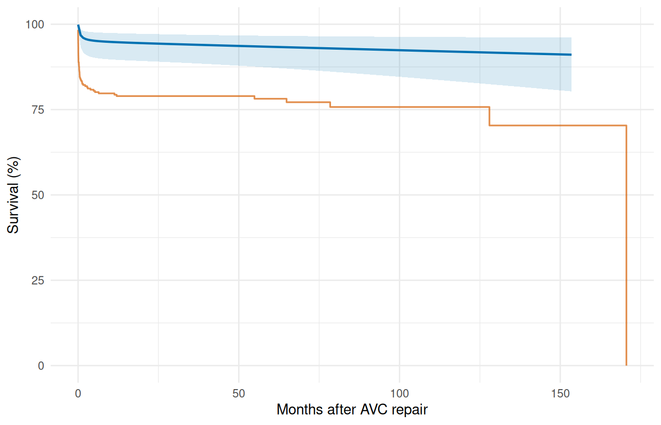

Figure 6: Reference patient survival with 95% delta-method CI and KM overlay

6.2 5b. Sensitivity analysis (risk factor comparison)

Coefficient tables tell you about effect direction and magnitude on the log-hazard scale. They don’t directly tell a clinician what to expect at the bedside. Sensitivity analysis closes that gap by scoring two clinically meaningful profiles (a low-risk patient drawn from the favorable end of each covariate, and a high-risk patient drawn from the unfavorable end) through the fitted model and plotting the resulting survival curves with delta-method confidence bands. The vertical and horizontal gaps between the two curves are the model’s clinical-impact statement, in the units (survival probability and time) that the audience actually recognizes.

low_risk <- data.frame(
  time   = t_grid,
  age    = quantile(avc$age, 0.25),
  status = 1,
  mal    = 0,
  com_iv = 0
)
#> Warning in data.frame(time = t_grid, age = quantile(avc$age, 0.25), status = 1,
#> : row names were found from a short variable and have been discarded

high_risk <- data.frame(
  time   = t_grid,
  age    = quantile(avc$age, 0.90),
  status = 4,
  mal    = 1,
  com_iv = 1
)
#> Warning in data.frame(time = t_grid, age = quantile(avc$age, 0.9), status = 4,
#> : row names were found from a short variable and have been discarded

surv_lo <- predict(fit_mv, newdata = low_risk,
                   type = "survival", se.fit = TRUE)
surv_hi <- predict(fit_mv, newdata = high_risk,
                   type = "survival", se.fit = TRUE)

sens_df <- data.frame(
  time     = rep(t_grid, 2),
  survival = c(surv_lo$fit, surv_hi$fit) * 100,
  lower    = c(surv_lo$lower, surv_hi$lower) * 100,
  upper    = c(surv_lo$upper, surv_hi$upper) * 100,
  profile  = rep(c("Low risk", "High risk"), each = length(t_grid))
)

ggplot(sens_df, aes(time, survival, colour = profile, fill = profile)) +
  geom_ribbon(aes(ymin = lower, ymax = upper),
              alpha = 0.15, colour = NA) +
  geom_line(linewidth = 0.8) +
  scale_colour_manual(values = c("Low risk" = "#0072B2",
                                  "High risk" = "#D55E00")) +
  scale_fill_manual(values = c("Low risk" = "#0072B2",
                                "High risk" = "#D55E00")) +
  labs(x = "Months after AVC repair", y = "Survival (%)",
       colour = NULL, fill = NULL) +
  coord_cartesian(ylim = c(0, 100)) +
  theme_minimal() +
  theme(legend.position = "bottom")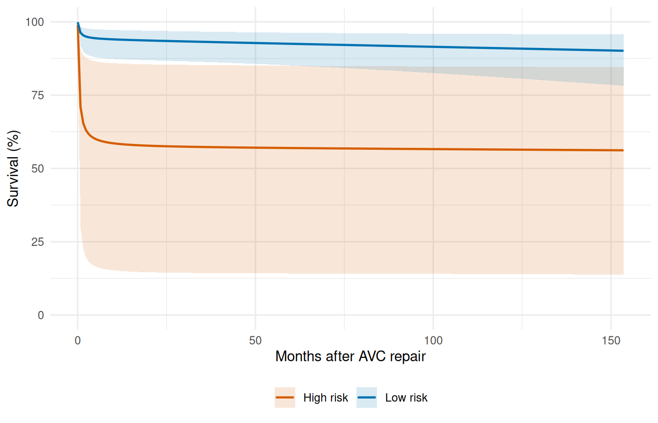

Figure 7: Survival by risk profile: low-risk (blue) vs. high-risk (orange)

Non-overlapping confidence bands between the two profiles indicate the risk-factor combination is well-identified; overlap around the bands’ centre-of-mass flags where the model can’t distinguish the profiles with the available sample size.

7 Step 6: Validation (decile-of-risk calibration)

Partition patients into deciles by predicted risk and compare observed vs. expected event rates. Good calibration means the two track each other. This implements the workflow of the SAS deciles.hazard.sas macro.

cal <- hzr_deciles(fit_mv, time = max(avc$int_dead))
print(cal)
#> Decile-of-risk calibration (risk grouped at time = 170.5826 )
#> 305 subjects, all included.
#> 10 groups, 68 observed events, 68 expected
#> 
#>  group  n events expected observed_rate expected_rate  chi_sq  p_value
#>      1 31      0     1.23        0.0000        0.0397  1.2300 0.267000
#>      2 30      0     1.57        0.0000        0.0525  1.5700 0.210000
#>      3 31      2     2.58        0.0645        0.0832  0.1300 0.718000
#>      4 30      3     3.30        0.1000        0.1100  0.0275 0.868000
#>      5 31      3     5.20        0.0968        0.1680  0.9280 0.335000
#>      6 30      6     6.74        0.2000        0.2250  0.0817 0.775000
#>      7 31     13     7.55        0.4190        0.2430  3.9400 0.047100
#>      8 30     17     7.26        0.5670        0.2420 13.1000 0.000303
#>      9 31     12    13.30        0.3870        0.4290  0.1290 0.720000
#>     10 30     12    19.30        0.4000        0.6420  2.7300 0.098200
#>  mean_survival mean_cumhaz
#>          0.943      0.0397
#>          0.923      0.0525
#>          0.881      0.0832
#>          0.849      0.1100
#>          0.793      0.1680
#>          0.750      0.2250
#>          0.673      0.2430
#>          0.605      0.2420
#>          0.525      0.4290
#>          0.308      0.6420
#> 
#> Overall: chi-sq = 23.8 on 9 df, p = 0.00459

ggplot(cal, aes(x = group)) +
  geom_col(aes(y = observed_rate), fill = "#56B4E9", alpha = 0.7) +
  geom_point(aes(y = expected_rate), colour = "#D55E00", size = 3) +
  geom_line(aes(y = expected_rate), colour = "#D55E00", linewidth = 0.5) +
  scale_x_continuous(breaks = seq_len(nrow(cal))) +
  labs(x = "Risk decile (1 = lowest)", y = "Event rate",
       caption = paste("Overall chi-sq =",
                        round(attr(cal, "overall")$chi_sq, 2),
                        ", p =",
                        format.pval(attr(cal, "overall")$p_value,
                                     digits = 3))) +
  theme_minimal()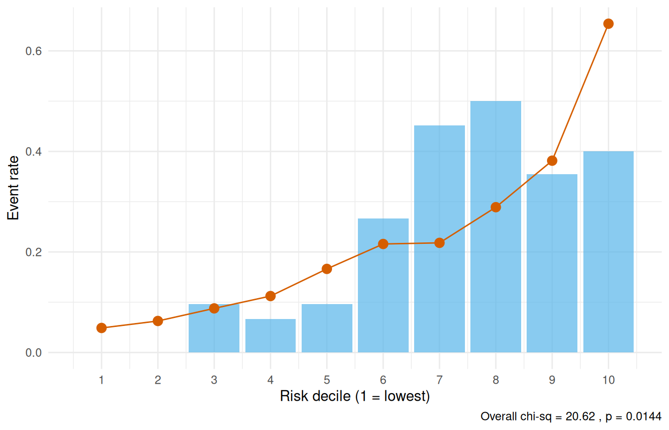

Figure 8: Decile calibration: observed (bars) vs. expected (points) event rates

A non-significant overall chi-square statistic (p > 0.05) means the test found no evidence of poor calibration. It does not prove the model is calibrated: with ten groups and few events in each, the test has little power. Read the plot as well. Calibration is adequate when the observed and expected rates track each other across the deciles.

7.1 Conservation of events check

The conservation-of-events principle says a model fit by maximum likelihood predicts as many events as were observed: add up every patient’s cumulative hazard at the end of their follow-up and you get the event count back. hzr_gof() is the R version of the SAS hazplot display, a running tally of observed and expected events over time. Each patient’s expected count is their own cumulative hazard, from their own covariates, at the time they leave follow-up.

gof <- hzr_gof(fit_mv)
print(gof)
#> Goodness-of-fit: observed vs. expected events
#> Distribution: multiphase  | n = 305 
#> 
#> Total observed events: 68 
#> Total expected events: 68 
#> Final residual (E - O): 0 
#> Conservation ratio (E/O): 1 
#> 
#> Use plot columns: time, km_surv, par_surv, cum_observed, cum_expected, residual

Expected 68.0 against 68 observed, an E/O of 1, so the fit conserves events. fit_mv is a multiphase fit with Conservation of Events applied (the default), which holds the total to the event count exactly. A Weibull fit gets there at its maximum, to within the optimizer’s tolerance.

ggplot(gof, aes(x = time)) +
  geom_step(aes(y = km_surv * 100), colour = "#D55E00", linewidth = 0.6) +
  geom_line(aes(y = par_surv * 100), colour = "#0072B2", linewidth = 0.8) +
  labs(x = "Months after AVC repair", y = "Survival (%)") +
  coord_cartesian(ylim = c(0, 100)) +
  theme_minimal()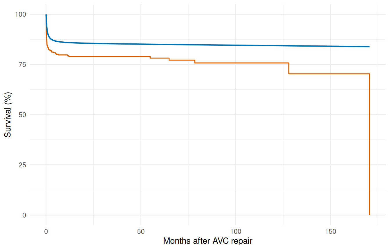

Figure 9: Parametric survival at the covariate means (blue) vs. Kaplan-Meier (orange)

ggplot(gof, aes(x = time)) +
  geom_line(aes(y = cum_observed), colour = "#D55E00", linewidth = 0.8) +
  geom_line(aes(y = cum_expected), colour = "#0072B2",
            linewidth = 0.8, linetype = "dashed") +
  labs(x = "Months after AVC repair", y = "Cumulative events") +
  theme_minimal()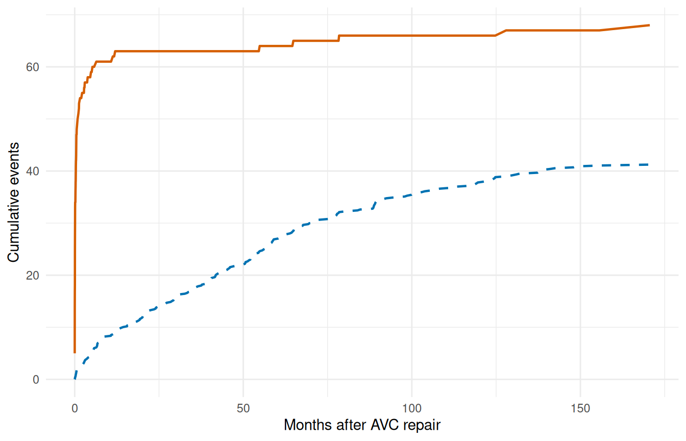

Figure 10: Cumulative observed (orange) vs. expected (blue) events

ggplot(gof, aes(x = time, y = residual)) +
  geom_line(linewidth = 0.7, colour = "grey30") +
  geom_hline(yintercept = 0, linetype = "dashed", colour = "grey60") +
  labs(x = "Months after AVC repair",
       y = "Residual (expected - observed)") +
  theme_minimal()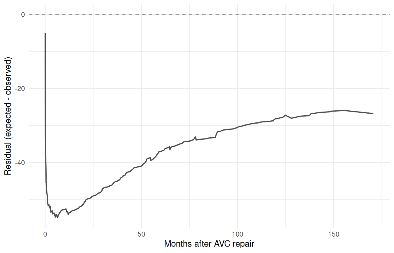

Figure 11: Conservation-of-events residual (expected minus observed) over time

The first plot is the one place the mean patient appears. It sets the survival curve for a patient with average covariates against the Kaplan-Meier estimate for the whole cohort, and that curve runs above it from the first weeks on. The mean patient fares better than the cohort, because the mean patient’s cumulative hazard is not the average of the patients’ cumulative hazards. That is why hzr_gof() builds its expected count patient by patient rather than from this curve.

The other two plots tally events as patients leave follow-up. A patient adds their expected count when they leave, by death or censoring, and that count is the hazard they built up over their whole follow-up. Most deaths come in the first weeks, to patients who had little time to build up hazard: 47 deaths in the first half month against about 4.8 expected. The residual bottoms out near -47.5 at about two months. The patients followed longest, most of them censored, carry the rest of the expected count, and it arrives only as they leave follow-up years later, so the residual climbs back and ends at zero. Read the shape of the curve as a record of when deaths and follow-up happen in this cohort, not as a month-by-month calibration check. The end point is the conservation-of-events identity, and the decile table above is the calibration check.

8 Why not Cox regression?

For this kind of analysis the temporal parametric approach buys you several things that Cox proportional hazards does not:

Feature	Cox (`coxph`)	TemporalHazard
Proportional hazards required	Yes	No
Baseline hazard specified	No	Yes (parametric)
Multiple hazard phases	No	Yes (additive)
Patient-specific survival curve	Step function (Breslow baseline)	Smooth, parametric
Smooth extrapolation beyond data	No	Yes
Conservation of events	Yes (martingale residuals sum to 0)	Yes (per-subject cumulative hazards sum to the event count)
Interval censoring	Not standard	Supported

Many clinical outcomes show non-proportional hazards: the risk factors that dominate early mortality (e.g., surgical complexity) differ from those driving late attrition (e.g., age, comorbidity). The multiphase model captures this through phase-specific covariate effects.

9 Summary

The complete analytical workflow follows a disciplined sequence:

Kaplan-Meier baseline: establish the empirical survival pattern
Shape fitting: match the temporal shape, simple to complex
Variable screening: logistic screening, decile-logit functional form
Multivariable model: enter covariates with fixed shapes
Prediction: reference curves, sensitivity analysis
Validation: decile calibration, conservation-of-events check

This sequence ensures that the temporal shape is established before covariates are introduced, and that the final model is validated against the observed data. See vignette("getting-started") for the minimal API workflow and vignette("mf-mathematical-foundations") for the mathematical details.