if (requireNamespace("hvtiRutilities", quietly = TRUE)) {
  library("hvtiRutilities")
} else {
  pkgload::load_all(export_all = FALSE, helpers = FALSE, quiet = TRUE)
}
#>
#>  hvtiRutilities 1.0.0.9004
#>
#>  Type hvtiRutilities.news() to see new features, changes, and bug fixes.
#>
library(labelled)Why Labels Matter
Variable labels are the bridge between raw data and human-readable output. A column named lvefvs_b means nothing in a table or plot caption, but “Baseline LV Ejection Fraction (%)” tells the reader exactly what they are looking at. In clinical research, where results go directly into manuscripts, grant submissions, and regulatory filings, unlabeled output is unprofessional and error-prone.
SAS datasets carry variable labels natively. When you import them into R with haven::read_sas(), the labelled package preserves those labels as column attributes. hvtiRutilities provides a set of functions to extract, look up, register, and override these labels throughout the analysis lifecycle.
The Label Lifecycle
A typical clinical analysis has four phases where labels matter:
- Ingestion — labels arrive with the data (SAS import) or need to be created (CSV import)
- Transformation — derived variables (ratios, bins, indices) need new labels
- Override — study-specific abbreviations or corrections
- Consumption — labels appear in plots, tables, and data dictionaries
Phase 1: Extracting Labels at Ingestion
label_map() extracts all variable labels into a lookup table:
# Simulated SAS-style dataset with labels
dta <- generate_survival_data(n = 200, seed = 42)

lmap <- label_map(dta)
head(lmap, 10)
#>                     key                                          label
#> ccfid             ccfid                                     Patient ID
#> origin_year origin_year                 Calendar year for iv_opyrs = 0
#> iv_opyrs       iv_opyrs Observation interval (years) since origin_year
#> iv_dead         iv_dead                Follow-up time to death (years)
#> dead               dead           Death indicator (1=dead, 0=censored)
#> reop               reop                      Reoperation (1=yes, 0=no)
#> iv_reop         iv_reop          Follow-up time to reoperation (years)
#> age                 age                         Age at surgery (years)
#> sex                 sex                                            Sex
#> bmi                 bmi                        Body mass index (kg/m2)
The result is a two-column data frame: key (variable name) and label (descriptive text). Every column in the data gets an entry. Unlabeled columns fall back to the variable name itself.
Detecting Missing Labels
When data arrives from a plain CSV (no labels), label_map() warns you:
csv_data <- data.frame(
  pat_id = 1:5,
  hgb = c(12.1, 14.3, 10.8, 13.5, 11.2),
  egfr = c(88, 72, 45, 91, 63)
)

# This triggers a warning --- most columns lack labels
lmap_csv <- label_map(csv_data)
#> Warning: 3 of 3 variables (100%) lack descriptive labels. Consider adding a
#> labels_overrides.yml or using add_labels().
print(lmap_csv)
#>           key  label
#> pat_id pat_id pat_id
#> hgb       hgb    hgb
#> egfr     egfr   egfr
The warning is intentional: it prevents the common mistake of generating plots and tables with cryptic variable names like hgb and egfr and not noticing until a collaborator asks what they mean.
Phase 2: Labeling Derived Variables
After ingestion, you’ll create new variables — age groups, risk scores, ratios, indicator flags. These variables have no labels because they didn’t exist in the original data.
Method A: Label the data directly (preferred)
The best practice is to label the data frame itself using add_labels(). Labels travel with the data through dplyr operations, so they are never out of sync:
# Create derived variables
dta$age_group <- cut(dta$age,
  breaks = c(0, 30, 50, 70, Inf),
  labels = c("<30", "30-50", "50-70", ">70")
)
dta$ef_low <- dta$lvefvs_b < 40

# Label them directly on the data frame
dta <- add_labels(dta, c(
  age_group = "Age Group at Surgery",
  ef_low    = "Reduced Ejection Fraction (<40%)"
))

# Verify
var_label(dta$age_group)
#> [1] "Age Group at Surgery"
var_label(dta$ef_low)
#> [1] "Reduced Ejection Fraction (<40%)"
When you label the data directly, any subsequent call to label_map() automatically picks up the new labels:
Method B: Update the label map (for reporting)
Sometimes the label map is created once and passed to a reporting module that generates tables and figures. In that case, update the map directly:
# Start from the base data
lmap <- label_map(generate_survival_data(n = 100, seed = 7))

# Register labels for variables you plan to create
lmap <- add_labels(lmap, c(
  age_group  = "Age Group at Surgery",
  ef_low     = "Reduced Ejection Fraction (<40%)",
  risk_score = "Composite Risk Score"
))

tail(lmap, 4)
#>                       key                            label
#> hypertension hypertension                     Hypertension
#> 1               age_group             Age Group at Surgery
#> 2                  ef_low Reduced Ejection Fraction (<40%)
#> 3              risk_score             Composite Risk Score
Which method should I use?
| Scenario | Method | Reason |
|---|---|---|
| Adding columns to a data frame | add_labels(data, ...) |
Labels travel with the data |
| Building a reporting table/dictionary | add_labels(lmap, ...) |
The map is the artifact being consumed |
| Quick lookup for a plot title | get_label(lmap, var) |
Safe, readable, errors on typos |
Phase 3: Study-Specific Overrides
Different studies use different abbreviations and naming conventions. An AVSD study might want “Common AVV” shortened to “CAVV”; a mitral valve study might need different terminology entirely. Hard-coding these replacements in shared functions is fragile.
apply_label_overrides() reads a YAML file and applies the overrides to a label map. If the file doesn’t exist, nothing happens — making it safe to call unconditionally.
# Create a study-specific overrides file
tmp_overrides <- tempfile(fileext = ".yml")
writeLines(c(
  "lvefvs_b: 'Baseline LVEF (%)'",
  "hgb_bs: 'Hemoglobin (g/dL)'",
  "gfr_bs: 'eGFR (mL/min/1.73m2)'",
  "nyha_class: 'NYHA Class'"
), tmp_overrides)

# Start with the default labels
lmap <- label_map(generate_survival_data(n = 50, seed = 1))

# Apply study-specific overrides
lmap <- apply_label_overrides(lmap, overrides_file = tmp_overrides)
lmap[lmap$key %in% c("lvefvs_b", "hgb_bs", "gfr_bs", "nyha_class"), ]
#>                   key                label
#> hgb_bs         hgb_bs    Hemoglobin (g/dL)
#> gfr_bs         gfr_bs eGFR (mL/min/1.73m2)
#> lvefvs_b     lvefvs_b    Baseline LVEF (%)
#> nyha_class nyha_class           NYHA Class
In a real project, labels_overrides.yml lives alongside config.yml in the project root and is committed to version control. Each study gets its own file; shared analysis code never contains hard-coded label replacements.
Example labels_overrides.yml
# AVSD study label overrides
cavv_area: "Common AVV Area (cm2)"
ed_area: "End-Diastolic Area (cm2)"
es_area: "End-Systolic Area (cm2)"
bsa_idx: "BSA-Indexed Value"
Phase 4: Using Labels in Output
Safe single-variable lookup with get_label()
The get_label() function replaces the error-prone match() pattern. It errors on typos instead of silently returning NA:
lmap <- label_map(generate_survival_data(n = 50, seed = 42))

# Use in plot titles
get_label(lmap, "age")
#> [1] "Age at surgery (years)"
get_label(lmap, "lvefvs_b")
#> [1] "Baseline LV ejection fraction (%)"
# Typo --- clear error instead of silent NA
get_label(lmap, "ages")
#> Error:
#> ! Variable 'ages' not found in label map.
Building a data dictionary
Use data_dictionary() to generate a complete, type-annotated data dictionary in one call:
dta <- generate_survival_data(n = 200, seed = 42)
dict <- data_dictionary(dta)
head(dict, 12)
#>                variable                                          label
#> ccfid             ccfid                                     Patient ID
#> origin_year origin_year                 Calendar year for iv_opyrs = 0
#> iv_opyrs       iv_opyrs Observation interval (years) since origin_year
#> iv_dead         iv_dead                Follow-up time to death (years)
#> dead               dead           Death indicator (1=dead, 0=censored)
#> reop               reop                      Reoperation (1=yes, 0=no)
#> iv_reop         iv_reop          Follow-up time to reoperation (years)
#> age                 age                         Age at surgery (years)
#> sex                 sex                                            Sex
#> bmi                 bmi                        Body mass index (kg/m2)
#> hgb_bs           hgb_bs                     Baseline hemoglobin (g/dL)
#> wbc_bs           wbc_bs                      Baseline WBC count (K/uL)
#>                 class n_unique pct_missing
#> ccfid       character      200         0.0
#> origin_year   integer       21         0.0
#> iv_opyrs      numeric      183         0.0
#> iv_dead       numeric      184         0.0
#> dead          integer        2         0.0
#> reop          integer        2         0.0
#> iv_reop       numeric       31        83.5
#> age           numeric      165         0.0
#> sex            factor        2         0.0
#> bmi           numeric      123         0.0
#> hgb_bs        numeric       66         0.0
#> wbc_bs        numeric      172         0.0
#>                                                                  summary
#> ccfid       200 levels: PT00001, PT00002, PT00003, PT00004, PT00005, ...
#> origin_year                                           1998 / 2008 / 2018
#> iv_opyrs                                             1.06 / 7.87 / 14.99
#> iv_dead                                               0.25 / 4.1 / 13.98
#> dead                                                           0 / 1 / 1
#> reop                                                           0 / 0 / 1
#> iv_reop                                               0.04 / 1.29 / 9.92
#> age                                                       1 / 44.75 / 85
#> sex                                               2 levels: Female, Male
#> bmi                                                    15 / 26.65 / 41.8
#> hgb_bs                                                     7.6 / 13 / 18
#> wbc_bs                                                1.5 / 7.35 / 15.53
Labels in summary tables
Use get_labels() (vectorized) to look up multiple labels at once:
lmap <- label_map(dta)
# Numeric summary with labels
num_vars <- c("age", "bmi", "hgb_bs", "gfr_bs", "lvefvs_b")
summary_tbl <- data.frame(
variable = num_vars,
label = get_labels(lmap, num_vars),
mean = vapply(num_vars, function(v) round(mean(dta[[v]]), 1), numeric(1)),
sd = vapply(num_vars, function(v) round(sd(dta[[v]]), 1), numeric(1)),
median = vapply(num_vars, function(v) round(median(dta[[v]]), 1), numeric(1))
)
print(summary_tbl)
#> variable label mean sd median
#> age age Age at surgery (years) 44.6 14.6 44.8
#> bmi bmi Body mass index (kg/m2) 26.8 4.8 26.6
#> hgb_bs hgb_bs Baseline hemoglobin (g/dL) 12.9 1.8 13.0
#> gfr_bs gfr_bs Baseline eGFR (mL/min/1.73m2) 76.2 19.4 75.8
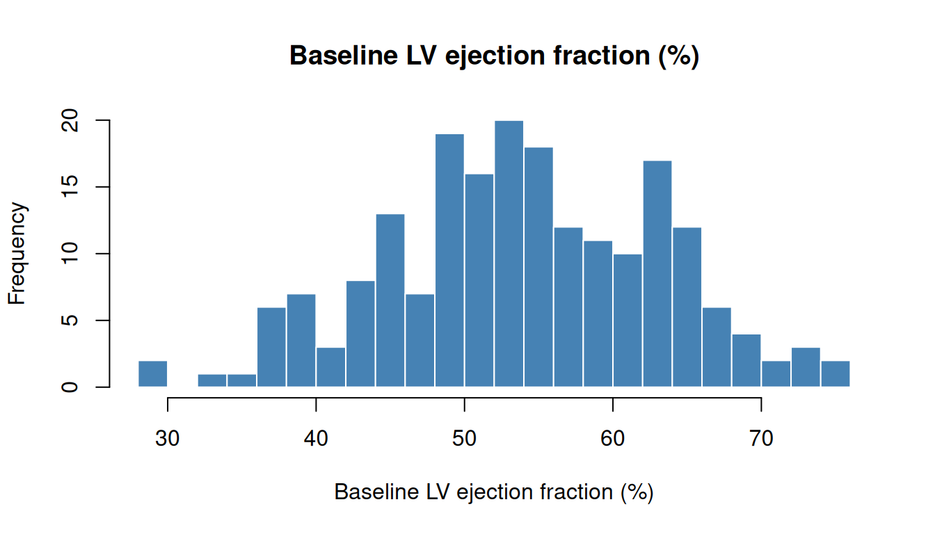
#> lvefvs_b lvefvs_b Baseline LV ejection fraction (%) 54.0 9.2 53.8Labels in plots
Complete Workflow
Putting it all together — a realistic analysis setup:
# 1. Load data (simulated here; in practice: haven::read_sas())
dta <- generate_survival_data(n = 500, seed = 2024)

# 2. Convert types
dta_clean <- r_data_types(dta,
  factor_size = 5,
  skip_vars   = c("ccfid", "iv_dead", "iv_reop", "iv_opyrs")
)

# 3. Create derived variables with labels
dta_clean$age_group <- cut(dta_clean$age,
  breaks = c(0, 30, 50, 70, Inf),
  labels = c("<30", "30-50", "50-70", ">70")
)
dta_clean$ef_category <- cut(dta_clean$lvefvs_b,
  breaks = c(0, 35, 50, Inf),
  labels = c("Reduced", "Borderline", "Normal")
)
dta_clean <- add_labels(dta_clean, c(
  age_group   = "Age Group at Surgery",
  ef_category = "Ejection Fraction Category"
))

# 4. Extract label map for reporting
lmap <- label_map(dta_clean)

# 5. Verify: all variables have real labels
stopifnot(!any(lmap$key == lmap$label))

# 6. Summary using labels
cat("Variables:", nrow(lmap), "\n")
#> Variables: 26
cat("All labeled:", !any(lmap$key == lmap$label), "\n")
#> All labeled: TRUE
head(lmap, 10)
#>                     key                                          label
#> ccfid             ccfid                                     Patient ID
#> origin_year origin_year                 Calendar year for iv_opyrs = 0
#> iv_opyrs       iv_opyrs Observation interval (years) since origin_year
#> iv_dead         iv_dead                Follow-up time to death (years)
#> dead               dead           Death indicator (1=dead, 0=censored)
#> reop               reop                      Reoperation (1=yes, 0=no)
#> iv_reop         iv_reop          Follow-up time to reoperation (years)
#> age                 age                         Age at surgery (years)
#> sex                 sex                                            Sex
#> bmi                 bmi                        Body mass index (kg/m2)
Labels and r_data_types()
Labels are preserved through type conversion. This is handled automatically — you don’t need to do anything special:
dta <- sample_data(n = 50)

# Before conversion
var_label(dta$char)
#> [1] "Gender"

# After conversion
dta_clean <- r_data_types(dta, skip_vars = "id")
var_label(dta_clean$char)
#> [1] "Gender"

# Labels survive the round-trip
lmap_before <- label_map(dta)
lmap_after  <- label_map(dta_clean)
identical(lmap_before, lmap_after)
#> [1] TRUE
Anti-Patterns to Avoid
1. Hard-coded label replacements in shared code
This breaks the moment anyone uses the code for a different study. Use apply_label_overrides() with a per-study YAML file instead.
2. Creating derived variables without labels
# BAD: new column has no label
dta$risk_score <- dta$age * 0.1 + as.integer(dta$nyha_class) * 0.5

# GOOD: label it immediately
dta$risk_score <- dta$age * 0.1 + as.integer(dta$nyha_class) * 0.5
dta <- add_labels(dta, c(risk_score = "Composite Risk Score"))
3. Using match() without error checking
4. Labeling the map instead of the data
# FRAGILE: map goes stale when you modify the data
dta$ratio <- dta$a / dta$b
lmap <- add_labels(lmap, c(ratio = "A/B Ratio"))
# ... 50 lines later, someone renames 'ratio' to 'ab_ratio'
# lmap still says "ratio" --- silent mismatch

# BETTER: label the data, extract the map later
dta$ratio <- dta$a / dta$b
dta <- add_labels(dta, c(ratio = "A/B Ratio"))
lmap <- label_map(dta)  # always in sync
Function Reference
| Function | Purpose |
|---|---|
label_map(data) |
Extract all labels into a lookup table |
get_label(lmap, var) |
Look up one label with error checking |
get_labels(lmap, vars) |
Look up multiple labels at once (vectorized) |
add_labels(data, labels) |
Label a data frame or update a label map |
apply_label_overrides(data, file) |
Apply study-specific overrides from YAML (works on label maps or data frames) |
data_dictionary(data) |
Build a type-annotated data dictionary |
Session Information
sessionInfo()
#> R version 4.5.3 (2026-03-11)
#> Platform: x86_64-pc-linux-gnu
#> Running under: Ubuntu 24.04.4 LTS
#>
#> Matrix products: default
#> BLAS:   /usr/lib/x86_64-linux-gnu/openblas-pthread/libblas.so.3
#> LAPACK: /usr/lib/x86_64-linux-gnu/openblas-pthread/libopenblasp-r0.3.26.so;  LAPACK version 3.12.0
#>
#> locale:
#>  [1] LC_CTYPE=C.UTF-8       LC_NUMERIC=C           LC_TIME=C.UTF-8
#>  [4] LC_COLLATE=C.UTF-8     LC_MONETARY=C.UTF-8    LC_MESSAGES=C.UTF-8
#>  [7] LC_PAPER=C.UTF-8       LC_NAME=C              LC_ADDRESS=C
#> [10] LC_TELEPHONE=C         LC_MEASUREMENT=C.UTF-8 LC_IDENTIFICATION=C
#>
#> time zone: UTC
#> tzcode source: system (glibc)
#>
#> attached base packages:
#> [1] stats     graphics  grDevices utils     datasets  methods   base
#>
#> other attached packages:
#> [1] labelled_2.16.0           hvtiRutilities_1.0.0.9004
#>
#> loaded via a namespace (and not attached):
#>  [1] vctrs_0.7.2      cli_3.6.5        knitr_1.51       rlang_1.1.7
#>  [5] xfun_0.57        forcats_1.0.1    haven_2.5.5      generics_0.1.4
#>  [9] jsonlite_2.0.0   glue_1.8.0       htmltools_0.5.9  hms_1.1.4
#> [13] rmarkdown_2.31   evaluate_1.0.5   tibble_3.3.1     fastmap_1.2.0
#> [17] yaml_2.3.12      lifecycle_1.0.5  compiler_4.5.3   dplyr_1.2.0
#> [21] pkgconfig_2.0.3  digest_0.6.39    R6_2.6.1         tidyselect_1.2.1
#> [25] pillar_1.11.1    magrittr_2.0.4   tools_4.5.3      withr_3.0.2