if (requireNamespace("hvtiRutilities", quietly = TRUE)) {
  library("hvtiRutilities")
} else {
  pkgload::load_all(export_all = FALSE, helpers = FALSE, quiet = TRUE)
}
#>
#>  hvtiRutilities 1.0.0.9004
#>
#>  Type hvtiRutilities.news() to see new features, changes, and bug fixes.
#> Overview
The generate_survival_data() function creates a realistic synthetic cardiac surgery cohort suitable for testing and demonstrating survival analysis workflows. Survival times are drawn from a Weibull distribution with a linear predictor built from clinical variables (LVEF, age, hemoglobin, NYHA class, eGFR), and administrative censoring is applied at up to 15 years.
Generating the Dataset
set.seed(42)
dta <- generate_survival_data(n = 500, seed = 1024)

dim(dta)
#> [1] 500  24
names(dta)
#>  [1] "ccfid"        "origin_year"  "iv_opyrs"     "iv_dead"      "dead"
#>  [6] "reop"         "iv_reop"      "age"          "sex"          "bmi"
#> [11] "hgb_bs"       "wbc_bs"       "plate_bs"     "gfr_bs"       "lvefvs_b"
#> [16] "lvmass_b"     "lvmsi_b"      "stvoli_b"     "stvold_b"     "bypass_time"
#> [21] "xclamp_time"  "nyha_class"   "diabetes"     "hypertension"
The dataset contains 24 columns covering patient identifiers, calendar anchors, survival outcomes, reoperation, demographics, pre-operative labs, cardiac function, and surgical variables.
Data Structure
str(dta)
#> 'data.frame':    500 obs. of  24 variables:
#>  $ ccfid       : chr  "PT00001" "PT00002" "PT00003" "PT00004" ...
#>   ..- attr(*, "label")= chr "Patient ID"
#>  $ origin_year : int  2002 2001 2018 1998 2007 2003 2011 2010 2003 2014 ...
#>   ..- attr(*, "label")= chr "Calendar year for iv_opyrs = 0"
#>  $ iv_opyrs    : num  5.13 4.03 10.51 12.84 3.17 ...
#>   ..- attr(*, "label")= chr "Observation interval (years) since origin_year"
#>  $ iv_dead     : num  5.13 4.03 10.51 12.84 3.17 ...
#>   ..- attr(*, "label")= chr "Follow-up time to death (years)"
#>  $ dead        : int  0 0 0 0 0 0 1 0 1 0 ...
#>   ..- attr(*, "label")= chr "Death indicator (1=dead, 0=censored)"
#>  $ reop        : int  0 0 1 0 1 0 0 0 0 0 ...
#>   ..- attr(*, "label")= chr "Reoperation (1=yes, 0=no)"
#>  $ iv_reop     : num  NA NA 4.37 NA 1.39 NA NA NA NA NA ...
#>   ..- attr(*, "label")= chr "Follow-up time to reoperation (years)"
#>  $ age         : num  33.3 39.2 14.5 30.3 48.7 13.4 39.3 76.1 60.4 52.1 ...
#>   ..- attr(*, "label")= chr "Age at surgery (years)"
#>  $ sex         : Factor w/ 2 levels "Female","Male": 1 1 1 1 1 2 2 1 1 1 ...
#>   ..- attr(*, "label")= chr "Sex"
#>  $ bmi         : num  33.3 25.9 28.5 29.2 20.8 25.3 34.3 26 19.2 27.2 ...
#>   ..- attr(*, "label")= chr "Body mass index (kg/m2)"
#>  $ hgb_bs      : num  15.3 10.1 15.4 11.7 9.8 9.8 9.6 15.7 15.7 13.1 ...
#>   ..- attr(*, "label")= chr "Baseline hemoglobin (g/dL)"
#>  $ wbc_bs      : num  1.5 10.37 3.29 6.37 10.99 ...
#>   ..- attr(*, "label")= chr "Baseline WBC count (K/uL)"
#>  $ plate_bs    : num  102 245 279 294 190 193 120 107 299 219 ...
#>   ..- attr(*, "label")= chr "Baseline platelet count (K/uL)"
#>  $ gfr_bs      : num  79.6 82.6 89 87 95.4 40.3 31.9 80.2 72.1 87.7 ...
#>   ..- attr(*, "label")= chr "Baseline eGFR (mL/min/1.73m2)"
#>  $ lvefvs_b    : num  56.8 58.3 67.9 55.1 62.6 59.3 55.8 58 75 41.8 ...
#>   ..- attr(*, "label")= chr "Baseline LV ejection fraction (%)"
#>  $ lvmass_b    : num  164 140 148 119 224 ...
#>   ..- attr(*, "label")= chr "Baseline LV mass (g)"
#>  $ lvmsi_b     : num  40 40 40 40 40 40 40 40 40 40 ...
#>   ..- attr(*, "label")= chr "Baseline LV mass index (g/m2)"
#>  $ stvoli_b    : num  74.1 30.9 35.9 62.6 59.2 55.7 62.9 64.1 76.3 66.2 ...
#>   ..- attr(*, "label")= chr "Baseline SV index - systolic (mL/m2)"
#>  $ stvold_b    : num  109.8 89.2 73.4 77.6 94.9 ...
#>   ..- attr(*, "label")= chr "Baseline SV index - diastolic (mL/m2)"
#>  $ bypass_time : num  102 92 47 79 75 34 51 44 110 72 ...
#>   ..- attr(*, "label")= chr "Cardiopulmonary bypass time (min)"
#>  $ xclamp_time : num  63 63 28 55 46 20 28 26 81 54 ...
#>   ..- attr(*, "label")= chr "Aortic cross-clamp time (min)"
#>  $ nyha_class  : Ord.factor w/ 4 levels "I"<"II"<"III"<..: 1 2 2 2 2 1 3 1 4 2 ...
#>   ..- attr(*, "label")= chr "NYHA functional class"
#>  $ diabetes    : Factor w/ 2 levels "No","Yes": 1 2 1 2 2 2 1 1 1 1 ...
#>   ..- attr(*, "label")= chr "Diabetes mellitus"
#>  $ hypertension: Factor w/ 2 levels "No","Yes": 2 1 1 1 1 1 1 2 1 2 ...
#>   ..- attr(*, "label")= chr "Hypertension"
Key columns:
| Column | Description |
|---|---|
ccfid |
Patient identifier |
origin_year |
Calendar year corresponding to iv_opyrs = 0
|
iv_opyrs |
Observation interval length (years) anchored at origin_year
|
iv_dead |
Observed follow-up time (years) |
dead |
Event indicator (1 = death, 0 = censored) |
reop |
Reoperation indicator |
iv_reop |
Time to reoperation (years; NA if no reoperation) |
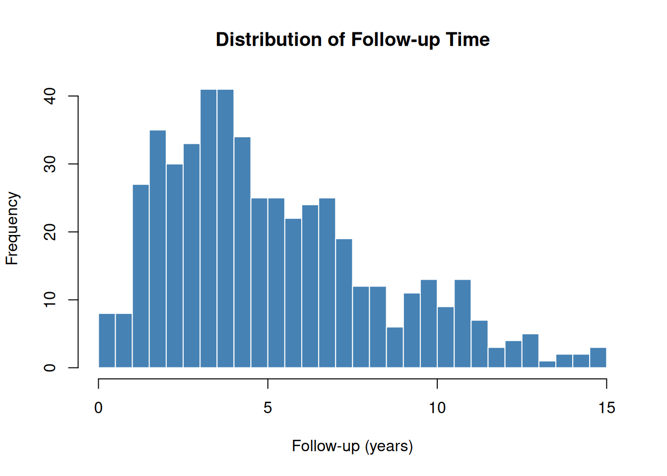
Outcome Summary
hist(
  dta$iv_dead,
  breaks = 30,
  main = "Distribution of Follow-up Time",
  xlab = "Follow-up (years)",
  col = "steelblue",
  border = "white"
)
Integration with r_data_types() and label_map()
The dataset arrives with variable labels attached and several columns that benefit from type conversion. The r_data_types() function handles these automatically.
# Convert types: keep IDs and continuous outcomes as-is
model_data <- r_data_types(
  dta,
  factor_size = 5,
  skip_vars = c("ccfid", "iv_dead", "iv_reop", "iv_opyrs")
)

str(model_data[, c("dead", "reop", "sex", "nyha_class", "diabetes", "hypertension")])
#> 'data.frame':    500 obs. of  6 variables:
#>  $ dead        : logi  FALSE FALSE FALSE FALSE FALSE FALSE ...
#>   ..- attr(*, "label")= chr "Death indicator (1=dead, 0=censored)"
#>  $ reop        : logi  FALSE FALSE TRUE FALSE TRUE FALSE ...
#>   ..- attr(*, "label")= chr "Reoperation (1=yes, 0=no)"
#>  $ sex         : Factor w/ 2 levels "Female","Male": 1 1 1 1 1 2 2 1 1 1 ...
#>   ..- attr(*, "label")= chr "Sex"
#>  $ nyha_class  : Ord.factor w/ 4 levels "I"<"II"<"III"<..: 1 2 2 2 2 1 3 1 4 2 ...
#>   ..- attr(*, "label")= chr "NYHA functional class"
#>  $ diabetes    : Factor w/ 2 levels "No","Yes": 1 2 1 2 2 2 1 1 1 1 ...
#>   ..- attr(*, "label")= chr "Diabetes mellitus"
#>  $ hypertension: Factor w/ 2 levels "No","Yes": 2 1 1 1 1 1 1 2 1 2 ...
#>   ..- attr(*, "label")= chr "Hypertension"
After conversion:
-
deadandreop(2 unique values) →logical -
sex,diabetes,hypertension(character) →factor -
nyha_classwas already an orderedfactor
Extracting Variable Labels
lmap <- label_map(model_data)
print(lmap)
#>                       key                                          label
#> ccfid               ccfid                                     Patient ID
#> origin_year   origin_year                 Calendar year for iv_opyrs = 0
#> iv_opyrs         iv_opyrs Observation interval (years) since origin_year
#> iv_dead           iv_dead                Follow-up time to death (years)
#> dead                 dead           Death indicator (1=dead, 0=censored)
#> reop                 reop                      Reoperation (1=yes, 0=no)
#> iv_reop           iv_reop          Follow-up time to reoperation (years)
#> age                   age                         Age at surgery (years)
#> sex                   sex                                            Sex
#> bmi                   bmi                        Body mass index (kg/m2)
#> hgb_bs             hgb_bs                     Baseline hemoglobin (g/dL)
#> wbc_bs             wbc_bs                      Baseline WBC count (K/uL)
#> plate_bs         plate_bs                 Baseline platelet count (K/uL)
#> gfr_bs             gfr_bs                  Baseline eGFR (mL/min/1.73m2)
#> lvefvs_b         lvefvs_b              Baseline LV ejection fraction (%)
#> lvmass_b         lvmass_b                           Baseline LV mass (g)
#> lvmsi_b           lvmsi_b                  Baseline LV mass index (g/m2)
#> stvoli_b         stvoli_b           Baseline SV index - systolic (mL/m2)
#> stvold_b         stvold_b          Baseline SV index - diastolic (mL/m2)
#> bypass_time   bypass_time              Cardiopulmonary bypass time (min)
#> xclamp_time   xclamp_time                  Aortic cross-clamp time (min)
#> nyha_class     nyha_class                          NYHA functional class
#> diabetes         diabetes                              Diabetes mellitus
#> hypertension hypertension                                   Hypertension
The label map is useful for annotating tables and plots with descriptive names.
Preparing Data for Survival Analysis
# Kaplan-Meier style summary by NYHA class (base R)
nyha_levels <- levels(model_data$nyha_class)

median_fu <- sapply(nyha_levels, function(lvl) {
  sub <- model_data[model_data$nyha_class == lvl, ]
  median(sub$iv_dead)
})

event_rate <- sapply(nyha_levels, function(lvl) {
  sub <- model_data[model_data$nyha_class == lvl, ]
  mean(sub$dead)
})

nyha_summary <- data.frame(
  nyha_class   = nyha_levels,
  n            = table(model_data$nyha_class),
  median_fu_yr = round(median_fu, 2),
  death_rate   = round(event_rate, 3)
)

print(nyha_summary)
#>     nyha_class n.Var1 n.Freq median_fu_yr death_rate
#> I            I      I    124         4.67      0.444
#> II          II     II    178         4.81      0.522
#> III        III    III    151         3.95      0.596
#> IV          IV     IV     47         3.45      0.681
Reproducibility
The seed argument ensures reproducible datasets for testing:
dta_a <- generate_survival_data(n = 100, seed = 99)
dta_b <- generate_survival_data(n = 100, seed = 99)

identical(dta_a, dta_b)  # TRUE
#> [1] TRUE
Different seeds produce different datasets:
dta_c <- generate_survival_data(n = 100, seed = 7)
identical(dta_a, dta_c)  # FALSE
#> [1] FALSE
Session Information
sessionInfo()
#> R version 4.5.3 (2026-03-11)
#> Platform: x86_64-pc-linux-gnu
#> Running under: Ubuntu 24.04.4 LTS
#>
#> Matrix products: default
#> BLAS:   /usr/lib/x86_64-linux-gnu/openblas-pthread/libblas.so.3
#> LAPACK: /usr/lib/x86_64-linux-gnu/openblas-pthread/libopenblasp-r0.3.26.so;  LAPACK version 3.12.0
#>
#> locale:
#>  [1] LC_CTYPE=C.UTF-8       LC_NUMERIC=C           LC_TIME=C.UTF-8
#>  [4] LC_COLLATE=C.UTF-8     LC_MONETARY=C.UTF-8    LC_MESSAGES=C.UTF-8
#>  [7] LC_PAPER=C.UTF-8       LC_NAME=C              LC_ADDRESS=C
#> [10] LC_TELEPHONE=C         LC_MEASUREMENT=C.UTF-8 LC_IDENTIFICATION=C
#>
#> time zone: UTC
#> tzcode source: system (glibc)
#>
#> attached base packages:
#> [1] stats     graphics  grDevices utils     datasets  methods   base
#>
#> other attached packages:
#> [1] hvtiRutilities_1.0.0.9004
#>
#> loaded via a namespace (and not attached):
#>  [1] vctrs_0.7.2      cli_3.6.5        knitr_1.51       rlang_1.1.7
#>  [5] xfun_0.57        forcats_1.0.1    haven_2.5.5      generics_0.1.4
#>  [9] jsonlite_2.0.0   glue_1.8.0       htmltools_0.5.9  hms_1.1.4
#> [13] rmarkdown_2.31   evaluate_1.0.5   tibble_3.3.1     fastmap_1.2.0
#> [17] yaml_2.3.12      lifecycle_1.0.5  compiler_4.5.3   dplyr_1.2.0
#> [21] pkgconfig_2.0.3  labelled_2.16.0  digest_0.6.39    R6_2.6.1
#> [25] tidyselect_1.2.1 pillar_1.11.1    magrittr_2.0.4   tools_4.5.3
#> [29] withr_3.0.2