Goodness-of-fit: observed vs. predicted events

Compare a fitted hazard model with the data two ways: its survival curve against the nonparametric Kaplan-Meier estimate, and the number of events it expects against the number observed, tallied over follow-up. This is the R equivalent of the SAS hazplot.sas macro and implements the conservation-of-events diagnostic.

Usage

hzr_gof(object, time_grid = NULL)

Arguments

object: A fitted hazard object (with fit = TRUE).
time_grid: Optional numeric vector of time points at which to evaluate the parametric model. If NULL (default), uses the distinct Kaplan-Meier times of the fitted data: the event and censoring times, with any closer together than survival::survfit()'s tolerance merged into one. A supplied grid must hold finite, non-negative times. It is sorted and exact repeats dropped, because the cumulative columns accumulate in time order.

Value

A data frame with one row per time point and columns:

time: Evaluation time.
n_risk: Number at risk at this time: subjects still in follow-up. A subject with an entry time is at risk only after it.
n_event: Number of events at this time.
n_censor: Number censored at this time.
km_surv: Kaplan-Meier survival estimate, using the counting-process risk set when the fit has entry times.
km_cumhaz: Kaplan-Meier cumulative hazard (\(-\log(\text{km\_surv})\)).
par_surv: Parametric survival from the fitted model, at the covariate means for a model with covariates. For plotting against km_surv; not used for cum_expected.
par_cumhaz: Parametric cumulative hazard, at the covariate means for a model with covariates. For plotting; not used for cum_expected.
cum_observed: Cumulative observed events to this time, weighted by the case weights for a weighted fit. With a custom time_grid, only the patients whose exit is a grid point up to this time are counted (see Details).
cum_expected: Cumulative expected events: over the patients leaving follow-up by this time (with a custom time_grid, the same patients as cum_observed), the sum of each patient's own cumulative hazard at exit minus that at entry, weighted by the case weights for a weighted fit. With time_windows, both cumulative hazards use the patient's covariate window at exit, as the likelihood does.
residual: Expected minus observed (cum_expected - cum_observed).

For multiphase models, additional columns are appended for each phase: par_cumhaz_<phase>, also at the covariate means.

An attribute "summary" is attached with scalar diagnostics: total observed events, total expected events, the final residual, and n_tallied, the number of patients the two tallies cover, out of n.

Details

The diagnostic is for right-censored data: every stored status must be 0 (censored) or 1 (event). A fit with any left-censored (status -1) or interval-censored (status 2) row is refused with an error. So is a multiphase fit that dropped the rows where a covariate was missing: its design matrices then hold fewer rows than there are patients, so no patient-by-patient tally can be formed. Refit it on complete cases.

At each time point the function computes:

The Kaplan-Meier survival and cumulative hazard.
The parametric survival and cumulative hazard from the fitted model at the covariate means (and per-phase components for multiphase models). This is the curve to plot against the Kaplan-Meier estimate.
Cumulative observed events vs. cumulative expected events. Each patient's expected count is their own cumulative hazard, from their own covariates, at the end of their follow-up, less their cumulative hazard at entry when the fit is left truncated (time_lower on a status 0 or 1 row). These are summed over the patients leaving follow-up at each time.
The running residual (expected minus observed).

The conservation-of-events principle says a model fit by maximum likelihood predicts as many events as were observed: add up every patient's cumulative hazard over their follow-up and you get the event count back. The final residual is then zero and the printed "Conservation ratio (E/O)" is 1. A multiphase fit with Conservation of Events applied (control = list(conserve = TRUE), the default) meets the identity by construction. Weibull and exponential fits meet it at the exact maximum, so at a converged fit E/O sits close to 1, off only by how far short of the maximum the optimizer stopped. The log-logistic and log-normal models carry no such identity, and for them E/O is a check of calibration in total.

The parametric curve is a different quantity. For a model with covariates it belongs to one "mean patient" with average covariates, and the mean patient's cumulative hazard is not the average of the patients' cumulative hazards, so par_cumhaz does not enter the expected count. For an intercept-only model every patient shares that curve. Without entry times each patient's expected count is the curve at their exit time; with entry times it is the curve's rise from entry to exit, so the two differ. The means are those of the design-matrix columns, taken phase by phase for a multiphase fit, whether its covariates enter globally, through the phase formulas or both, so a factor enters as the proportion of patients in each level. With time_windows, a phase built on the global covariates carries their means in the window that contains each time; a phase formula's own columns keep their plain means.

For a weighted fit both tallies carry the case weights: observed events are \(\sum_i w_i d_i\) and expected events \(\sum_i w_i H_i\), the form in which a weighted fit conserves events. The n_risk, n_event, n_censor and Kaplan-Meier columns are unweighted.

Each patient is placed at the Kaplan-Meier time survival::survfit() gives them, which merges exit times closer together than its tolerance. On the default grid every patient lands on a grid point, and hzr_gof() warns if one cannot be placed. With a custom time_grid, a patient is counted in both tallies only if that time, or failing it their own follow-up time, falls on a grid point. A grid such as seq() over the follow-up holds few exit times, so hzr_gof() warns with the number left out, and the totals, residual and E/O then describe only the patients counted. Include the exit times in time_grid to count everyone.

Examples

# \donttest{
data(avc)
avc <- na.omit(avc)
fit <- hazard(
  survival::Surv(int_dead, dead) ~ age + mal,
  data  = avc,
  dist  = "weibull",
  theta = c(mu = 0.01, nu = 0.5, beta_age = 0, beta_mal = 0),
  fit   = TRUE
)
gof <- hzr_gof(fit)
print(gof)
#> Goodness-of-fit: observed vs. expected events
#> Distribution: weibull  | n = 305 
#> 
#> Total observed events: 68 
#> Total expected events: 67.999 
#> Final residual (E - O): -0.001 
#> Conservation ratio (E/O): 1 
#> 
#> Use plot columns: time, km_surv, par_surv, cum_observed, cum_expected, residual

# Expected events are summed per patient.  This fit has no entry times,
# so the total is the sum of each patient's own cumulative hazard at
# their follow-up time:
nd <- avc[, c("age", "mal")]
nd$time <- avc$int_dead
c(hzr_gof = attr(gof, "summary")$total_expected,
  predict = sum(predict(fit, newdata = nd, type = "cumulative_hazard")))
#> hzr_gof predict 
#> 67.9993 67.9993 

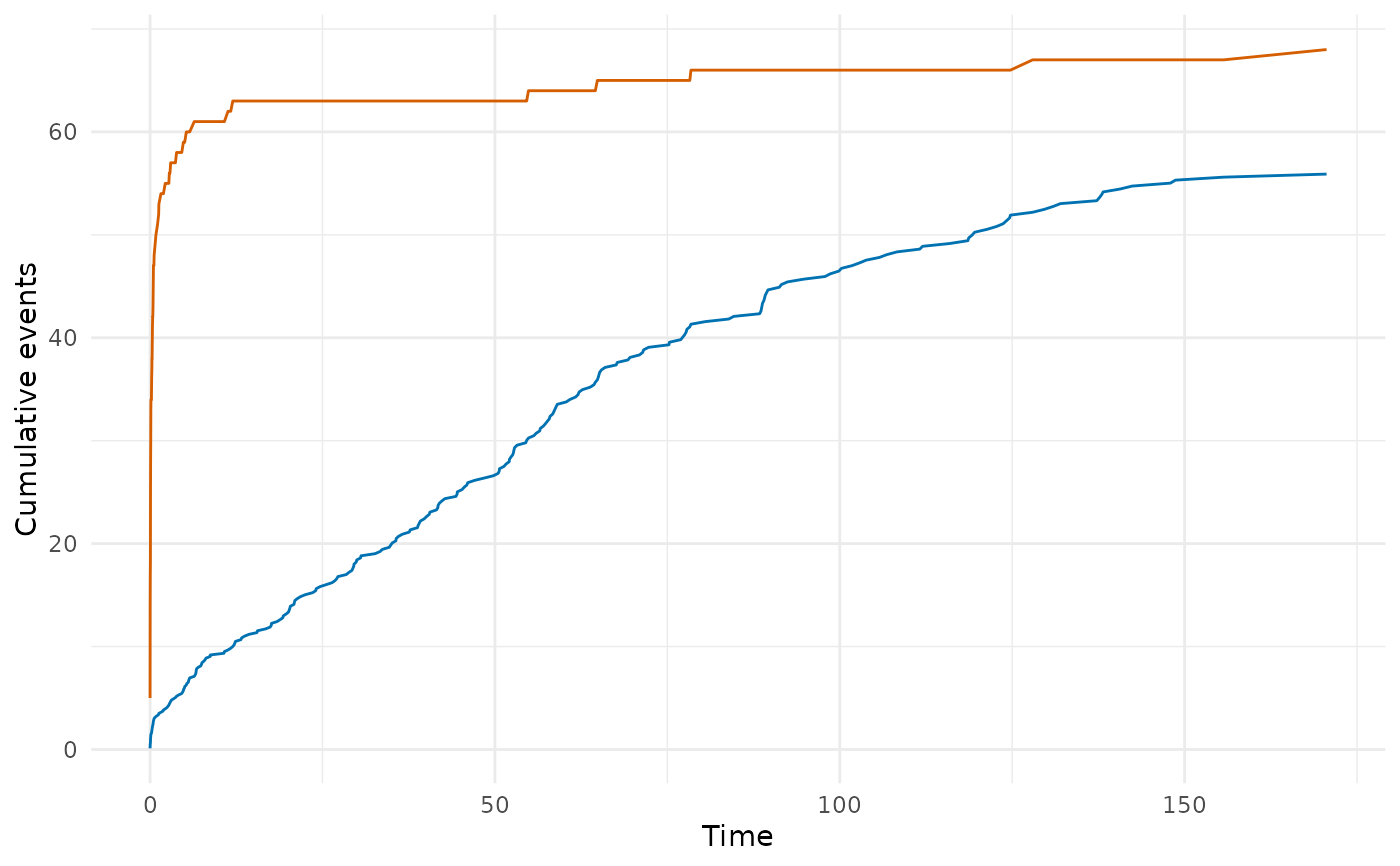
# Plot observed vs expected events
if (requireNamespace("ggplot2", quietly = TRUE)) {
  library(ggplot2)
  ggplot(gof, aes(x = time)) +
    geom_line(aes(y = cum_observed), colour = "#D55E00") +
    geom_line(aes(y = cum_expected), colour = "#0072B2") +
    labs(x = "Time", y = "Cumulative events") +
    theme_minimal()
}

# }

Usage

Arguments

Value

Details

See also

Examples