Prepare a scatter-plot matrix

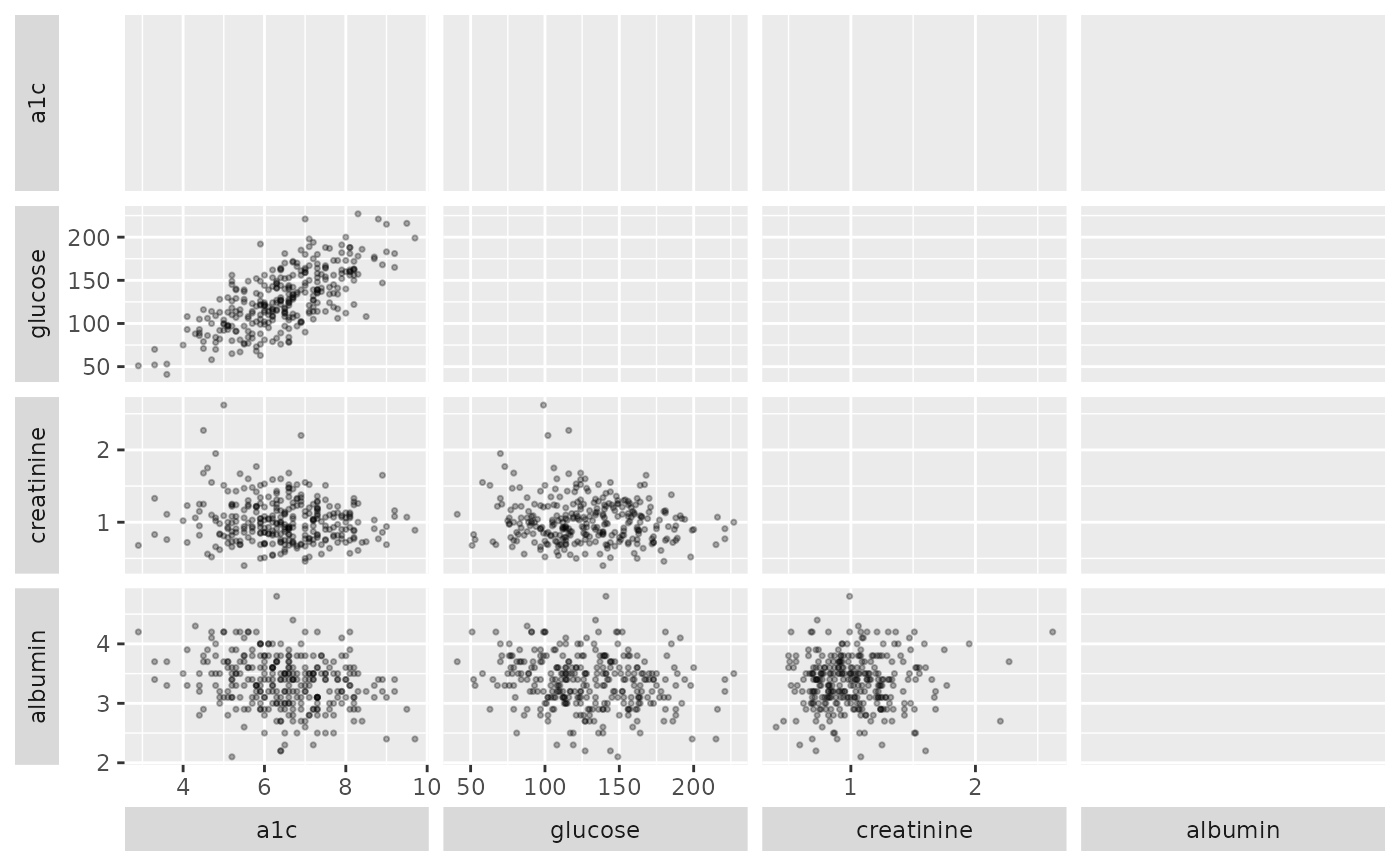
The scatter-plot-matrix analogue of SAS proc corr ... plots=matrix: one scatter panel per unordered pair of vars, lower triangle only. It is the plot half of the dc-tables job in the hvtiR job catalog. Call plot() on the result for a bare ggplot; the coefficient table with Fisher intervals is hvtiRtables::hv_correlation_table().

Usage

hv_correlation_matrix(
  data,
  vars,
  labels = NULL,
  method = c("pearson", "spearman")
)

Arguments

data: Data frame; one row per patient.
vars: Character vector of at least two numeric columns, in display order.
labels: Optional character vector of display labels, one per vars.
method: Coefficient stored in $tables$coefficients: "pearson" or "spearman".

Value

An object of class c("hv_correlation_matrix", "hv_data"): $data (columns col_var, row_var, x, y), $meta (vars, labels, method, n_obs, which is nrow(data) before any pairwise deletion, not a per-panel count), and $tables$coefficients, the pairwise coefficient matrix.

Details

Rows missing either coordinate are dropped panel by panel (pairwise deletion, as proc corr does), so a variable with missing values thins only the panels it appears in.

A single warning() names variables with fewer than 3 non-missing values or no variation, and otherwise-usable pairs with fewer than 3 pairwise-complete observations. These panels are sparse or flat, so their coefficients may be unstable or NA.

At large sizes (about 73 MB at 17 variables by 11,000 rows), write a raster format such as PNG rather than PDF, since every point is a vector object in a PDF, and lower alpha so overplotted panels stay legible.

References

SAS template: descriptive/dc.tables.ods.sas.

Examples

d <- sample_correlation_data()
cm <- hv_correlation_matrix(d, c("a1c", "glucose", "creatinine", "albumin"))
plot(cm) + theme_hv_manuscript()

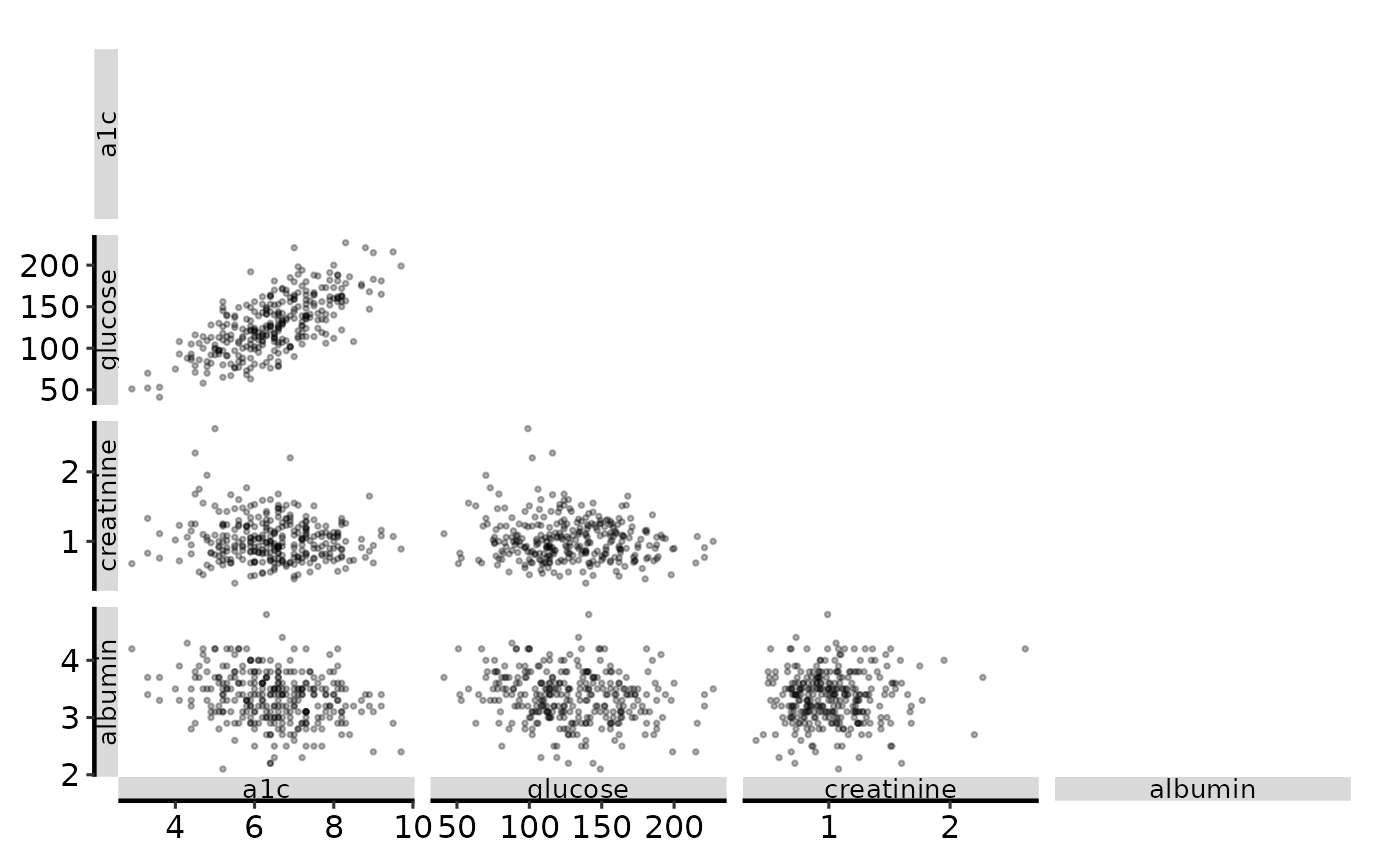# strip.placement moves the variable names outside the axis
plot(cm) + ggplot2::theme(strip.placement = "outside")