Prepare a paginated EDA section

Classifies each variable with eda_classify_var(), keeps the ones that belong to section, and prepares one hv_eda() panel for each. Call plot.hv_eda_pages() on the result to lay the panels out as pages.

Usage

hv_eda_pages(
  data,
  x_col = "year",
  section = c("continuous", "percent", "count"),
  vars = NULL,
  labels = NULL,
  unique_limit = 6L,
  unique_bound = 100,
  type_overrides = NULL
)

Arguments

data

Data frame; one row per patient.

x_col

Name of the reference column, usually the year of operation. Default "year".

section

One of "continuous", "percent" or "count".

vars

Character vector of the variables to consider, in page order. NULL (the default) means every column except x_col and any whose name marks a patient identifier: ccfid, patid, patientid, studyid, subjectid, recordid or caseid (each also with _, num or no), or mrn as a word of the name (mrn, mrn_num, pt_mrn, but not bnp_mrna). Such a column is not a study variable: drawn, it is a scatter of row numbers or a bar chart with one level per patient. meta$ignored lists what was left out; name a column here to draw it. Every name is checked at once, and the error lists all that are missing.

labels

Optional named character vector of display labels, names being column names. A variable without a label is shown by its name.

unique_limit, unique_bound, type_overrides

Passed to eda_classify_var().

Value

An object of class c("hv_eda_pages", "hv_data"):

$data

One row per variable in the section, in page order: variable, label, var_type.

$meta

Named list: x_col, section, x_binned, n_vars, n_obs, n_other, the number of considered variables that belong to other sections, and ignored, the identifier columns vars = NULL left out.

$tables

panels, a named list of hv_eda() objects, one per variable.

Details

The three sections split one dataset by variable class:

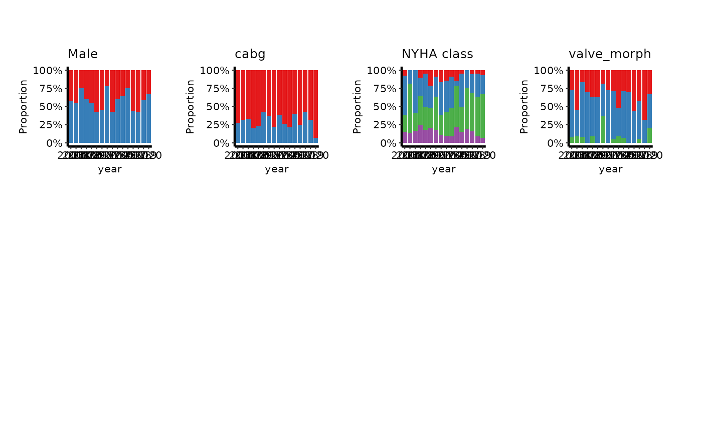
• "continuous": variables classified "Cont", drawn as scatter plots against x_col.

• "percent": categorical variables ("Cat_Num", "Cat_Char"), drawn as bars filled to 100% in each bin of x_col.

• "count": the same categorical variables, drawn as stacked counts.

The percent and count sections use the same bins. Categorical panels need a discrete x, so x_col is binned once, here, and every categorical panel reads that bin. A whole-valued x_col (a calendar year) is used as it is. A fractional one (years since an origin) is binned by floor(), so each bar is one whole year, and meta$x_binned records that it was. Continuous panels always use x_col unbinned.

See also

plot.hv_eda_pages(), hv_eda(), eda_classify_var()

Examples

dta <- sample_eda_data(n = 300, seed = 42)

# Continuous variables, four panels to a page
cont <- hv_eda_pages(dta, x_col = "year", section = "continuous")
cont
#> <hv_eda_pages>
#>   Section     : continuous
#>   Variables   : 4 (4 in other sections)
#>   x col       : year
#>   N obs       : 300
pages <- plot(cont, ncol = 2, nrow = 2)
length(pages)
#> [1] 1
attr(pages[[1]], "variables")
#> [1] "op_years"  "ef"        "lv_mass"   "peak_grad"

# Categorical variables as percentages, decorated across the whole page
pct <- hv_eda_pages(dta, x_col = "year", section = "percent",
                    labels = c(male = "Male", nyha = "NYHA class"))
plot(pct)[[1]] &
  ggplot2::scale_fill_brewer(palette = "Set1", na.value = "gray80") &
  theme_hv_manuscript(base_size = 8)