Validates and stores pre-computed parametric curve data — and optional
Kaplan-Meier empirical overlay and population life-table reference — as an
hv_hazard object. Pass the result to plot.hv_hazard() to render
the figure.
Usage
hv_hazard(
  curve_data,
  x_col = "time",
  estimate_col = "survival",
  lower_col = NULL,
  upper_col = NULL,
  group_col = NULL,
  empirical = NULL,
  emp_x_col = x_col,
  emp_estimate_col = "estimate",
  emp_lower_col = NULL,
  emp_upper_col = NULL,
  emp_group_col = group_col,
  emp_geom = c("point", "step"),
  reference = NULL,
  ref_x_col = x_col,
  ref_estimate_col = estimate_col,
  ref_group_col = NULL
)
Arguments
- curve_data
Data frame of parametric predictions (fine grid). Typical source: SAS
predictdataset exported to CSV, orsample_hazard_data().- x_col
Name of the time / age column. Default
"time".- estimate_col
Name of the predicted-value column:
"survival","hazard", or"cumhaz". Default"survival".- lower_col
Lower CI column in
curve_data, orNULLfor no ribbon. DefaultNULL.- upper_col
Upper CI column in
curve_data, orNULL. DefaultNULL.- group_col
Stratification column in
curve_data, orNULLfor a single curve. DefaultNULL.- empirical
Optional data frame of KM empirical points (SAS
ploutdataset). Stored in$tables$empirical. DefaultNULL.- emp_x_col
x column in
empirical. Defaults tox_col.- emp_estimate_col
y column in
empirical. Default"estimate".- emp_lower_col
Lower error-bar column in
empirical, orNULL. DefaultNULL.- emp_upper_col
Upper error-bar column in
empirical, orNULL. DefaultNULL.- emp_group_col
Group column in
empirical. Defaults togroup_col.- emp_geom
Geom used for the empirical overlay:
"point"(default, open circles) or"step"(Kaplan-Meier step function).- reference
Optional data frame of population life-table curves (SAS
smatcheddataset). Stored in$tables$reference. DefaultNULL.- ref_x_col
x column in
reference. Defaults tox_col.- ref_estimate_col
y column in
reference. Defaults toestimate_col.- ref_group_col
Linetype-grouping column in
reference, orNULL. DefaultNULL.
Value
An S3 object of class c("hv_hazard", "hv_data"); call
plot() on the result to render — see plot.hv_hazard(). The object
contains: $data (curve data frame), $meta (all column-name mappings),
$tables$empirical, $tables$reference.
Details
This constructor covers the complete tp.hp.dead.* SAS template family.
All column-name mappings and all three data frames are fixed at construction
time; aesthetic parameters (ci_alpha, line_width, etc.) are passed to
plot().
See also
plot.hv_hazard() to render as a ggplot2 figure,
theme_hv_manuscript() for the publication theme,
sample_hazard_data(), sample_hazard_empirical(),
sample_life_table() for example data.
Other Hazard plot:
plot.hv_hazard()
Examples
library(ggplot2)
dat <- sample_hazard_data(n = 500, time_max = 10)
emp <- sample_hazard_empirical(n = 500, time_max = 10, n_bins = 6)
# 1. Build data object
hp <- hv_hazard(dat,
lower_col = "surv_lower", upper_col = "surv_upper",
empirical = emp,
emp_lower_col = "lower", emp_upper_col = "upper"
)
hp # prints CI and empirical flags
#> <hv_hazard>
#> x col : time
#> estimate : survival
#> CI : surv_lower -- surv_upper
#> $data : 500 rows × 10 cols
#> $empirical : 6 rows
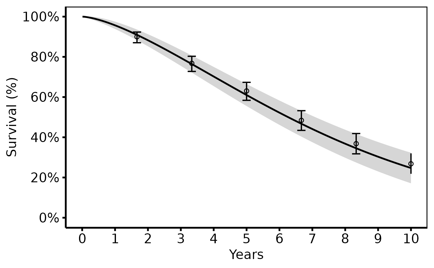
# 2. Bare plot -- undecorated ggplot returned by plot.hv_hazard
p <- plot(hp)
# 3. Decorate: colour/fill palettes, axis scales, labels, theme
p +
scale_colour_manual(values = c("steelblue"), guide = "none") +
scale_fill_manual(values = c("steelblue"), guide = "none") +
scale_x_continuous(limits = c(0, 10), breaks = 0:10) +
scale_y_continuous(limits = c(0, 100), breaks = seq(0, 100, 20),
labels = function(x) paste0(x, "%")) +
labs(x = "Years", y = "Survival (%)") +
theme_hv_poster()
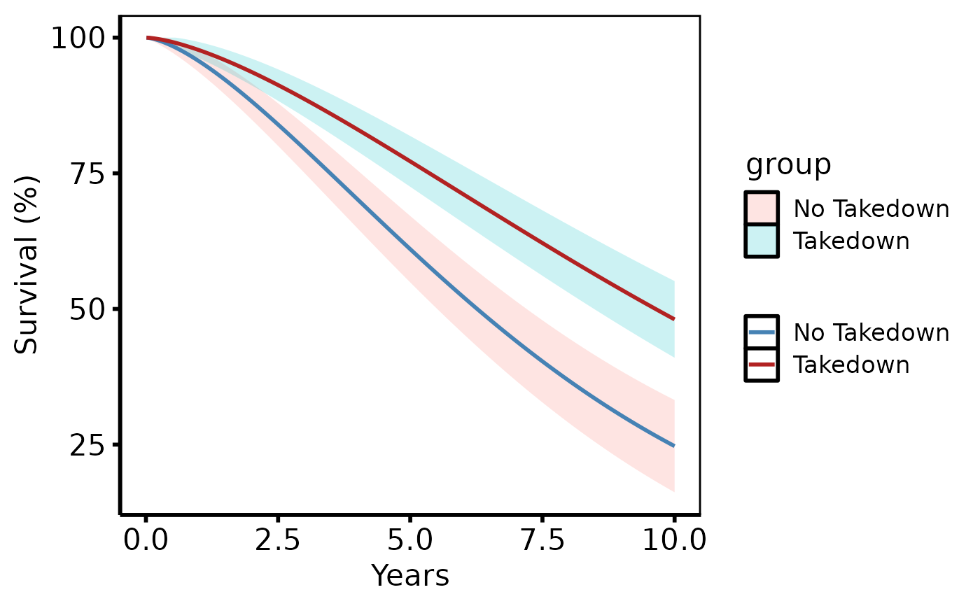
 # Stratified groups -- colour scale adds clinical meaning
dat2 <- sample_hazard_data(
n = 400, groups = c("No Takedown" = 1.0, "Takedown" = 0.65)
)
hp2 <- hv_hazard(dat2,
lower_col = "surv_lower", upper_col = "surv_upper",
group_col = "group"
)
plot(hp2) +
scale_colour_manual(
values = c("No Takedown" = "steelblue", "Takedown" = "firebrick"),
name = NULL
) +
labs(x = "Years", y = "Survival (%)") +
theme_hv_poster()
# Stratified groups -- colour scale adds clinical meaning
dat2 <- sample_hazard_data(
n = 400, groups = c("No Takedown" = 1.0, "Takedown" = 0.65)
)
hp2 <- hv_hazard(dat2,
lower_col = "surv_lower", upper_col = "surv_upper",
group_col = "group"
)
plot(hp2) +
scale_colour_manual(
values = c("No Takedown" = "steelblue", "Takedown" = "firebrick"),
name = NULL
) +
labs(x = "Years", y = "Survival (%)") +
theme_hv_poster()
 # --- Global theme + RColorBrewer (set once per session) ------------------
if (FALSE) { # \dontrun{
old <- ggplot2::theme_set(theme_hv_manuscript())
plot(hp2) +
scale_colour_brewer(palette = "Set1", name = NULL) +
scale_fill_brewer(palette = "Set1", guide = "none") +
scale_x_continuous(limits = c(0, 10), breaks = 0:10) +
scale_y_continuous(limits = c(0, 100), breaks = seq(0, 100, 20),
labels = function(x) paste0(x, "%")) +
labs(x = "Years", y = "Survival (%)")
ggplot2::theme_set(old)
} # }
# See vignette("plot-decorators", package = "hvtiPlotR") for theming,
# colour scales, annotation labels, and saving plots.
# --- Global theme + RColorBrewer (set once per session) ------------------
if (FALSE) { # \dontrun{
old <- ggplot2::theme_set(theme_hv_manuscript())
plot(hp2) +
scale_colour_brewer(palette = "Set1", name = NULL) +
scale_fill_brewer(palette = "Set1", guide = "none") +
scale_x_continuous(limits = c(0, 10), breaks = 0:10) +
scale_y_continuous(limits = c(0, 100), breaks = seq(0, 100, 20),
labels = function(x) paste0(x, "%")) +
labs(x = "Years", y = "Survival (%)")
ggplot2::theme_set(old)
} # }
# See vignette("plot-decorators", package = "hvtiPlotR") for theming,
# colour scales, annotation labels, and saving plots.