Plot an hv_survival object

Builds a bare ggplot2 object from an hv_survival data object. The plot contains the correct aesthetics and geometries but no scale, label, or theme modifications — add those with + as you would with any ggplot2 object.

Usage

# S3 method for class 'hv_survival'
plot(
  x,
  type = c("survival", "cumhaz", "hazard", "loglog", "life"),
  conf_int = TRUE,
  alpha = 0.8,
  ...
)

Arguments

x

An hv_survival object.

type

Which plot variant to produce. One of:

"survival"

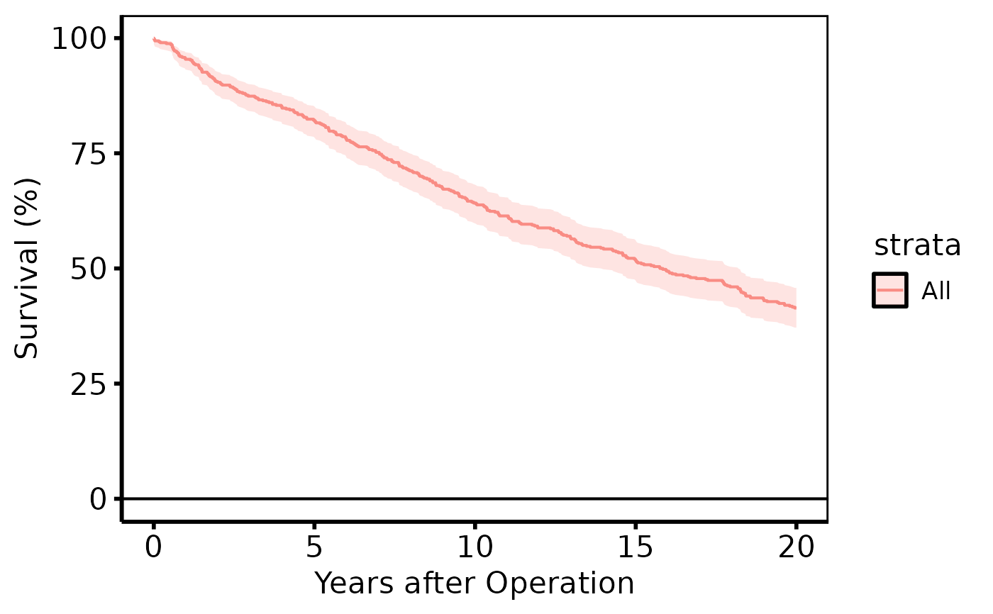
(default, PLOTS=1) KM step function with optional CI ribbon; y-axis on the 0–100 percent scale.

"cumhaz"

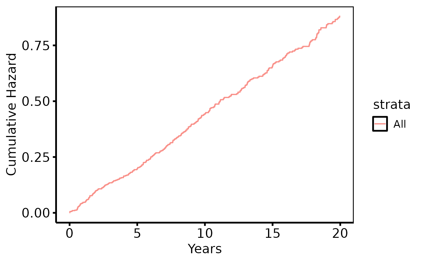
(PLOTC=1) Nelson-Aalen cumulative hazard \(H(t) = -\log S(t)\).

"hazard"

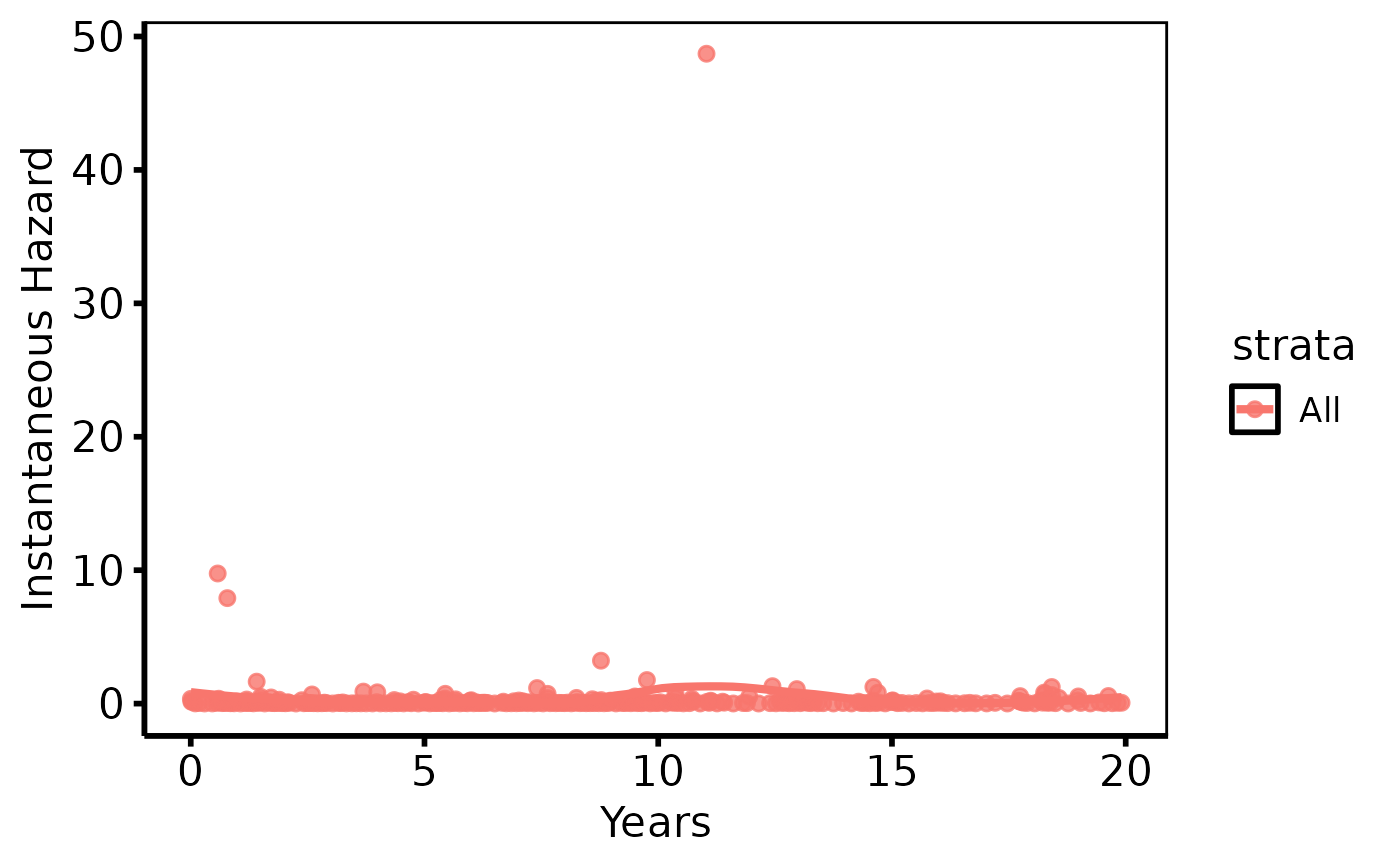
(PLOTH=1) Instantaneous hazard \(h(t)\); add geom_smooth(method="loess") for a smoothed publication curve.

"loglog"

Log-log diagnostic: \(\log H(t)\) vs \(\log t\). Parallel lines across strata support proportional hazards.

"life"

(PLOTL=1) Restricted mean survival time (integral of \(S(t)\)) vs time.

conf_int

Logical; draw a CI ribbon on the "survival" plot. Default TRUE. Ignored for other type values.

alpha

Line/point transparency in \([0,1]\). Default 0.8.

...

Ignored; present for S3 consistency.

Value

A bare ggplot object; compose with + to add scales, axis limits, labels, and hv_theme.

See also

hv_survival to build the data object, hv_theme for the publication theme.

Other Kaplan-Meier survival: hv_survival()

Examples

dta <- sample_survival_data(n = 500, seed = 42)
km  <- hv_survival(dta)

# Default survival curve
plot(km) +
  ggplot2::labs(x = "Years after Operation", y = "Survival (%)") +
  hv_theme("poster")


# Cumulative hazard
plot(km, type = "cumhaz") +
  ggplot2::labs(x = "Years", y = "Cumulative Hazard") +
  hv_theme("poster")


# Hazard rate with loess smoother
plot(km, type = "hazard") +
  ggplot2::geom_smooth(
    ggplot2::aes(x = .data[["mid_time"]], y = .data[["hazard"]]),
    method = "loess", se = FALSE, span = 0.5
  ) +
  ggplot2::labs(x = "Years", y = "Instantaneous Hazard") +
  hv_theme("poster")
#> `geom_smooth()` using formula = 'y ~ x'