A fitted random forest carries a lot of information, but getting at it usually means digging through list structures that were never meant to be plotted directly. ggRandomForests does that digging for you: it pulls tidy data objects out of a randomForestSRC or randomForest fit, and those objects drop straight into the ggplot2 workflows you already know. A second engine, varPro, powers a parallel family of functions for release-rule importance and related diagnostics; that family is covered in the companion vignette referenced at the end. This vignette walks through the three objects you will reach for most often (gg_error, gg_variable, and gg_vimp), plus a small helper for cutting a predictor into evenly populated groups.
Error trajectories with gg_error()
Type rfNews() to see new features/changes/bug fixes.
set.seed(42)
rf_iris <- randomForest(Species ~ ., data = iris, ntree = 200, keep.forest = TRUE)
err_df <- ggRandomForests::gg_error(rf_iris, training = TRUE)
head(err_df)
<gg_error> from randomForest | family: classification | ntree: 200 | n: 150
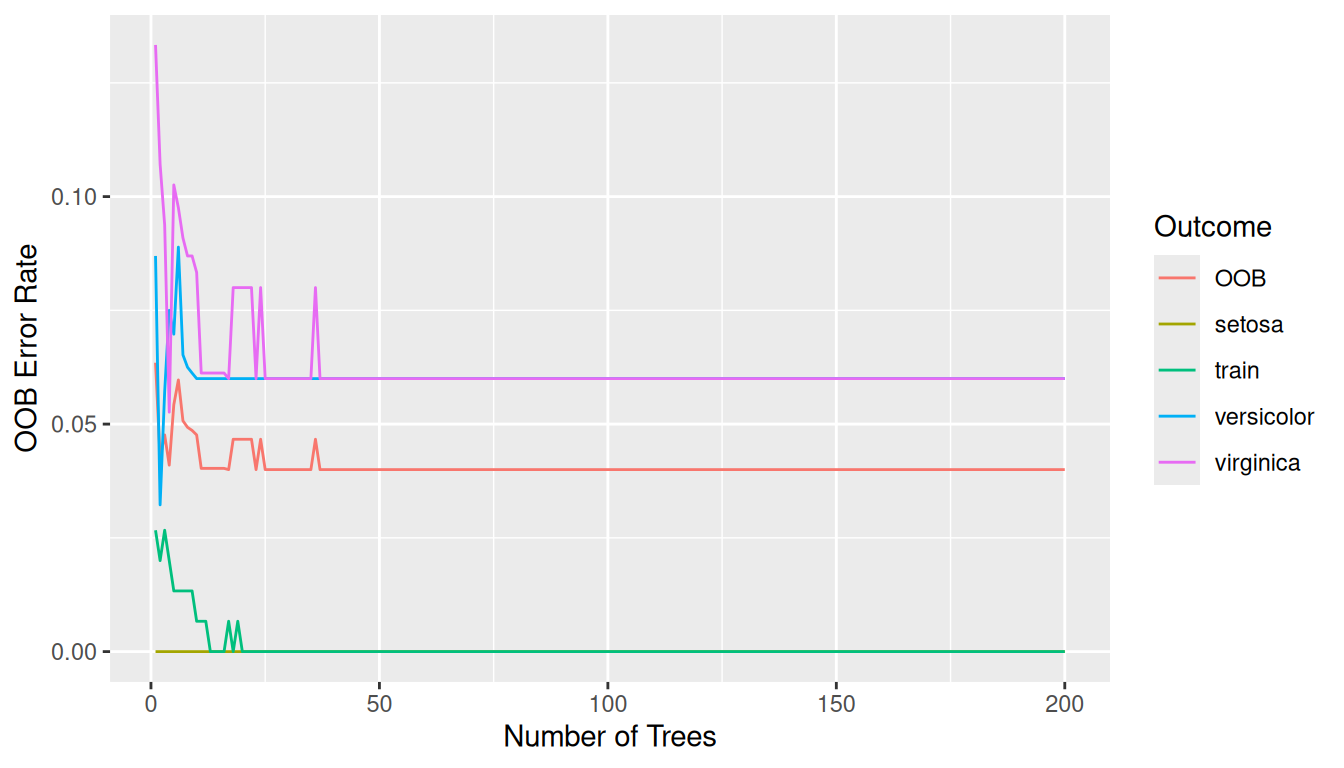
A forest’s error rate settles down as trees are added, and the gg_error() object lets you watch that happen. It holds the cumulative out-of-bag (OOB) error rate for each outcome column, indexed by the ntree counter. Ask for training = TRUE and the function reconstructs the original model frame and adds the in-bag error trajectory (train) as well, so you can see both curves at once:
Marginal dependence via gg_variable()
Classes 'gg_variable', 'regression' and 'data.frame':   506 obs. of  2 variables:
 $ lstat: num  4.98 9.14 4.03 2.94 5.33 ...
 $ yhat : num  29.2 22.5 35.1 36.4 33.4 ...
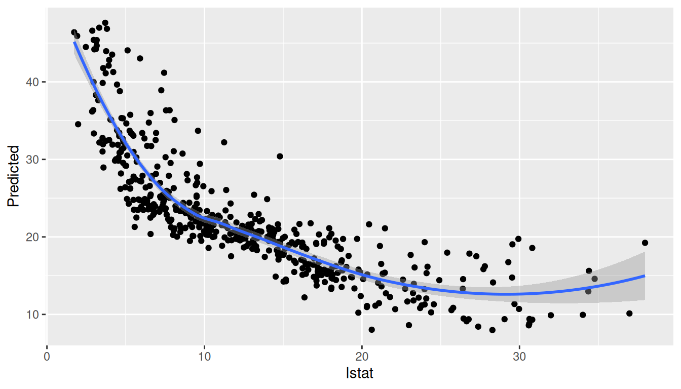
gg_variable() recovers the training data straight from the model call, so it still works when the forest was fit inside a helper function or against a subset() expression, cases where the data is not sitting in the global environment. The object you get back keeps the raw predictors alongside the prediction: a single yhat column for regression, or one yhat.<class> column per class for classification. To plot one predictor, name it with xvar:
plot(var_df, xvar = "lstat")
`geom_smooth()` using method = 'loess' and formula = 'y ~ x'
Survival forests can request multiple horizons using the time argument; non-OOB predictions are available by setting oob = FALSE.
Variable importance with gg_vimp()
vimp_df <- ggRandomForests::gg_vimp(rf_boston)
head(vimp_df)
<gg_vimp> from randomForest | family: regression | ntree: 150 | n: 506 | variables: 6
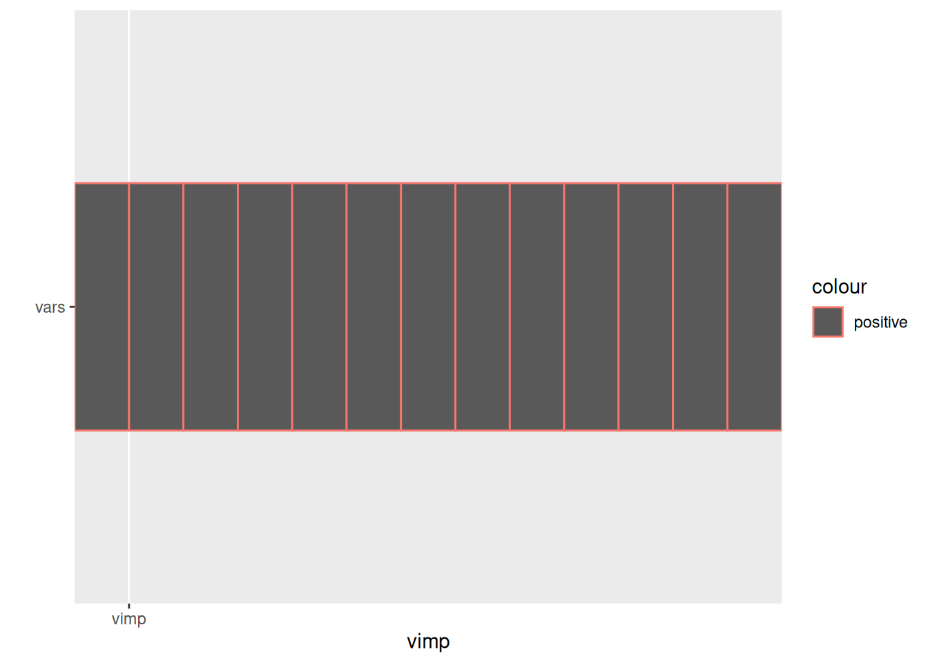
gg_vimp() measures permutation importance: each predictor is permuted in turn, and the drop in OOB accuracy gives its score. This contrasts with the gg_varpro family, which uses release-rule importance from the varPro engine. Variable importance is not always stored on the fitted object. If a randomForest fit is missing its importance scores, gg_vimp() will try to compute them for you. When even that is not possible (the forest was grown with importance = FALSE and the predictors are no longer reachable), the function warns and returns NA in place of the scores, so a plot still draws rather than failing outright.
Balanced conditioning cuts with quantile_pts()
rm_breaks <- ggRandomForests::quantile_pts(boston$rm, groups = 6, intervals = TRUE)
rm_groups <- cut(boston$rm, breaks = rm_breaks)
table(rm_groups)
rm_groups
(3.56,5.76] (5.76,5.99] (5.99,6.21] (6.21,6.44] (6.44,6.85] (6.85,8.78]
         85          84          84          85          84          84
When you build a coplot, you want each conditioning group to hold a roughly equal share of the data — equal-width bins leave the sparse tails nearly empty. quantile_pts() wraps stats::quantile() to give you break points that do exactly that, and they pass straight to cut() for the grouping or facet labels.
Next steps
- The full API reference lives at https://ehrlinger.github.io/ggRandomForests/.
-
?gg_error, ?gg_variable, ?gg_vimp, and ?quantile_pts cover the remaining arguments and have their own examples.
- The
gg_error, gg_variable, and gg_vimp objects shown here are tidy data frames underneath, so you can skip the plot() methods entirely and build the figure yourself with ggplot2.
- For the full varPro toolkit (release-rule importance, lasso-refined importance, per-observation local importance, anomaly scores, and the dependency graph) walked across regression, classification, and survival examples, see
vignette("varpro", package = "ggRandomForests").