plot.variable generates a
data.frame containing the marginal variable dependence or the
partial variable dependence. The gg_variable function creates a
data.frame of containing the full set of covariate data (predictor
variables) and the predicted response for each observation. Marginal
dependence figures are created using the plot.gg_variable
function.
A randomForest fit does not keep the model frame, so for those
objects gg_variable rebuilds it from the stored call. That lets the
same predictors be paired with the in-sample predictions.
A few optional arguments tune the extraction: time (one survival
time, or a vector of them), time_labels (labels for multiple
survival horizons), and oob, which switches between out-of-bag and
in-bag predictions when the forest carries both.
Arguments
- object
A
rfsrcorrandomForestobject, or aplot.variableresult.- ...
Optional arguments
time,time_labels, andoobthat tune the marginal dependence extraction.
Value
A gg_variable object: a data.frame pairing every
training predictor column with the OOB (or in-bag) predicted response.
For survival forests, each requested time horizon adds a column named by
time_labels. The object carries a "family" class attribute
("regr", "class", or "surv") that
plot.gg_variable uses for dispatch.
Details
The marginal variable dependence is determined by comparing relation between the predicted response from the randomForest and a covariate of interest.
The gg_variable function operates on a
rfsrc object, the output from the
plot.variable function, or on a fitted
randomForest object via the formula interface.
Examples
## ------------------------------------------------------------
## classification (small, runs on CRAN)
## ------------------------------------------------------------
## -------- iris data
set.seed(42)
rfsrc_iris <- randomForestSRC::rfsrc(Species ~ ., data = iris, ntree = 50)
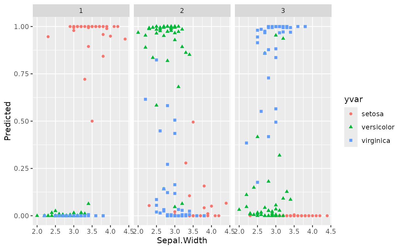
gg_dta <- gg_variable(rfsrc_iris)
plot(gg_dta, xvar = "Sepal.Width")
#> `geom_smooth()` using method = 'loess' and formula = 'y ~ x'
 # \donttest{
## ------------------------------------------------------------
## Additional classification / regression / survival examples are
## guarded with \donttest because the cumulative example time exceeds
## the 10-second CRAN budget. Run locally with `R CMD check
## --run-donttest` (or `devtools::check(run_dont_test = TRUE)`) to
## exercise them.
## ------------------------------------------------------------
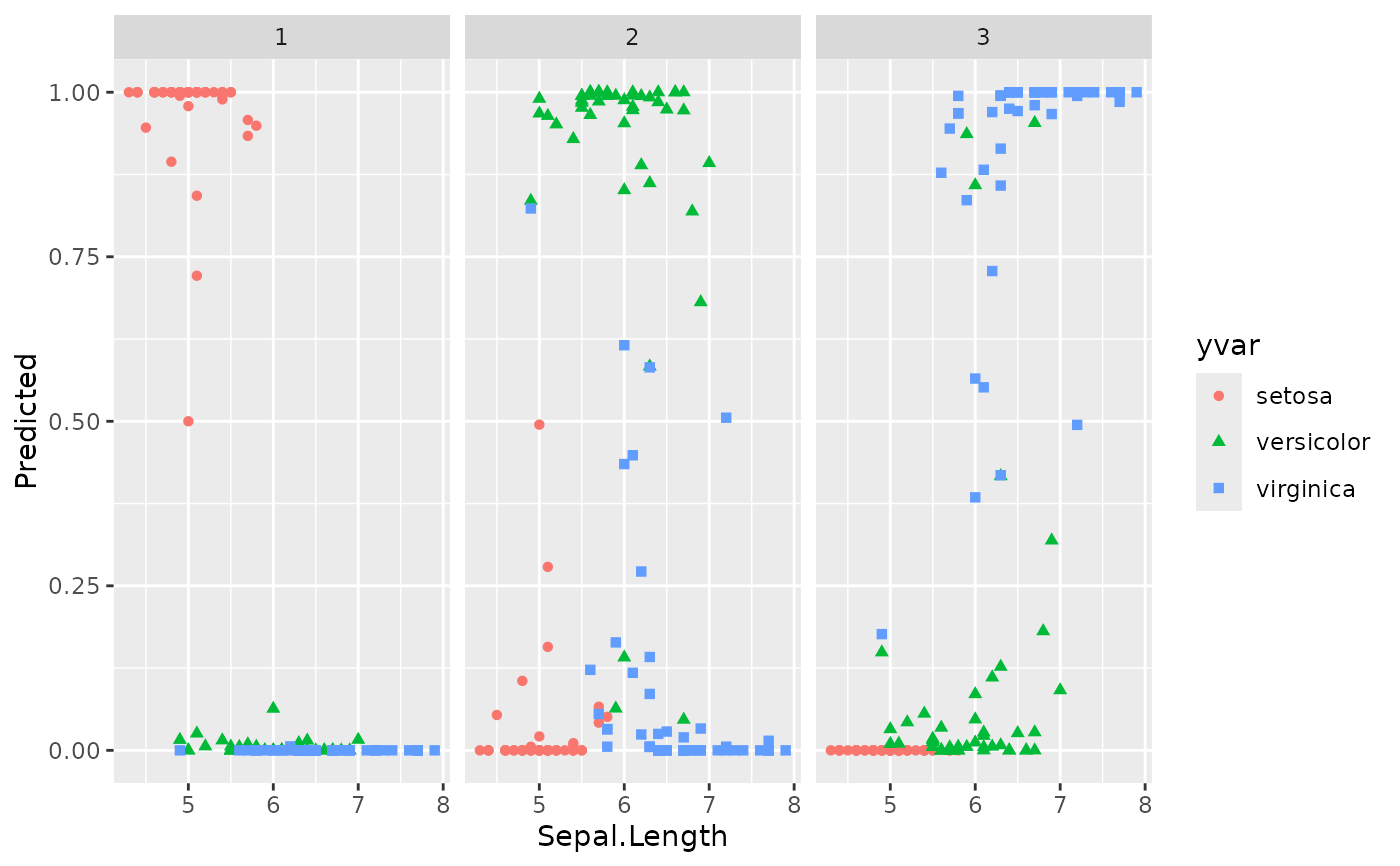
plot(gg_dta, xvar = "Sepal.Length")
#> `geom_smooth()` using method = 'loess' and formula = 'y ~ x'
# \donttest{
## ------------------------------------------------------------
## Additional classification / regression / survival examples are
## guarded with \donttest because the cumulative example time exceeds
## the 10-second CRAN budget. Run locally with `R CMD check
## --run-donttest` (or `devtools::check(run_dont_test = TRUE)`) to
## exercise them.
## ------------------------------------------------------------
plot(gg_dta, xvar = "Sepal.Length")
#> `geom_smooth()` using method = 'loess' and formula = 'y ~ x'
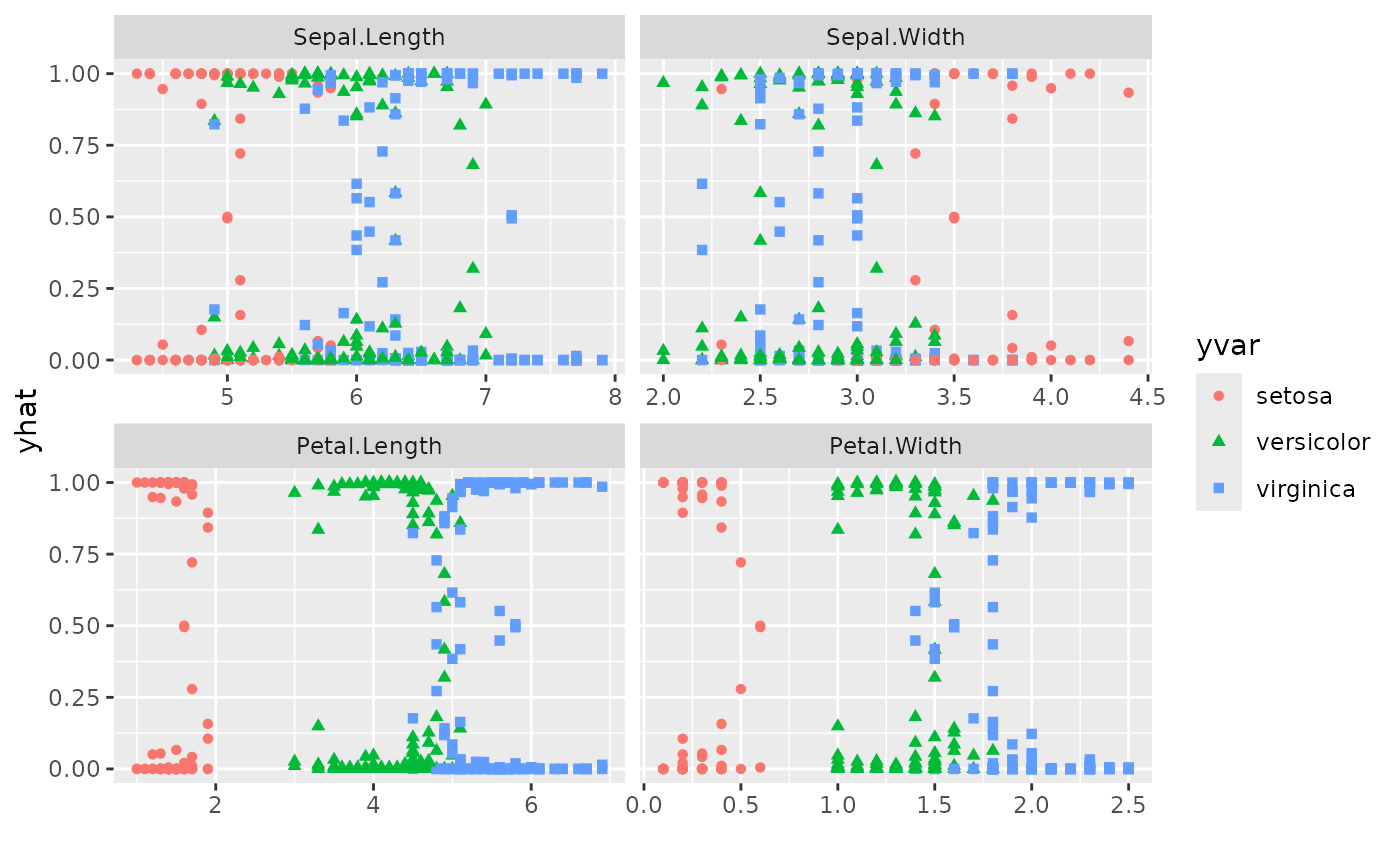
 plot(gg_dta, xvar = rfsrc_iris$xvar.names, panel = TRUE)
 ## ------------------------------------------------------------
## regression
## ------------------------------------------------------------
## -------- air quality data
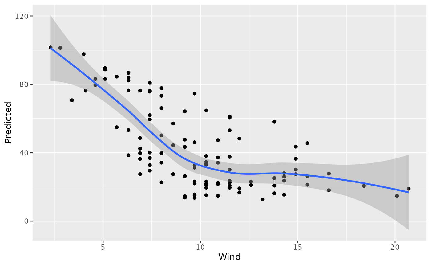
rfsrc_airq <- randomForestSRC::rfsrc(Ozone ~ ., data = airquality, ntree = 50)
gg_dta <- gg_variable(rfsrc_airq)
# an ordinal variable
gg_dta[, "Month"] <- factor(gg_dta[, "Month"])
plot(gg_dta, xvar = "Wind")
#> `geom_smooth()` using method = 'loess' and formula = 'y ~ x'
## ------------------------------------------------------------
## regression
## ------------------------------------------------------------
## -------- air quality data
rfsrc_airq <- randomForestSRC::rfsrc(Ozone ~ ., data = airquality, ntree = 50)
gg_dta <- gg_variable(rfsrc_airq)
# an ordinal variable
gg_dta[, "Month"] <- factor(gg_dta[, "Month"])
plot(gg_dta, xvar = "Wind")
#> `geom_smooth()` using method = 'loess' and formula = 'y ~ x'
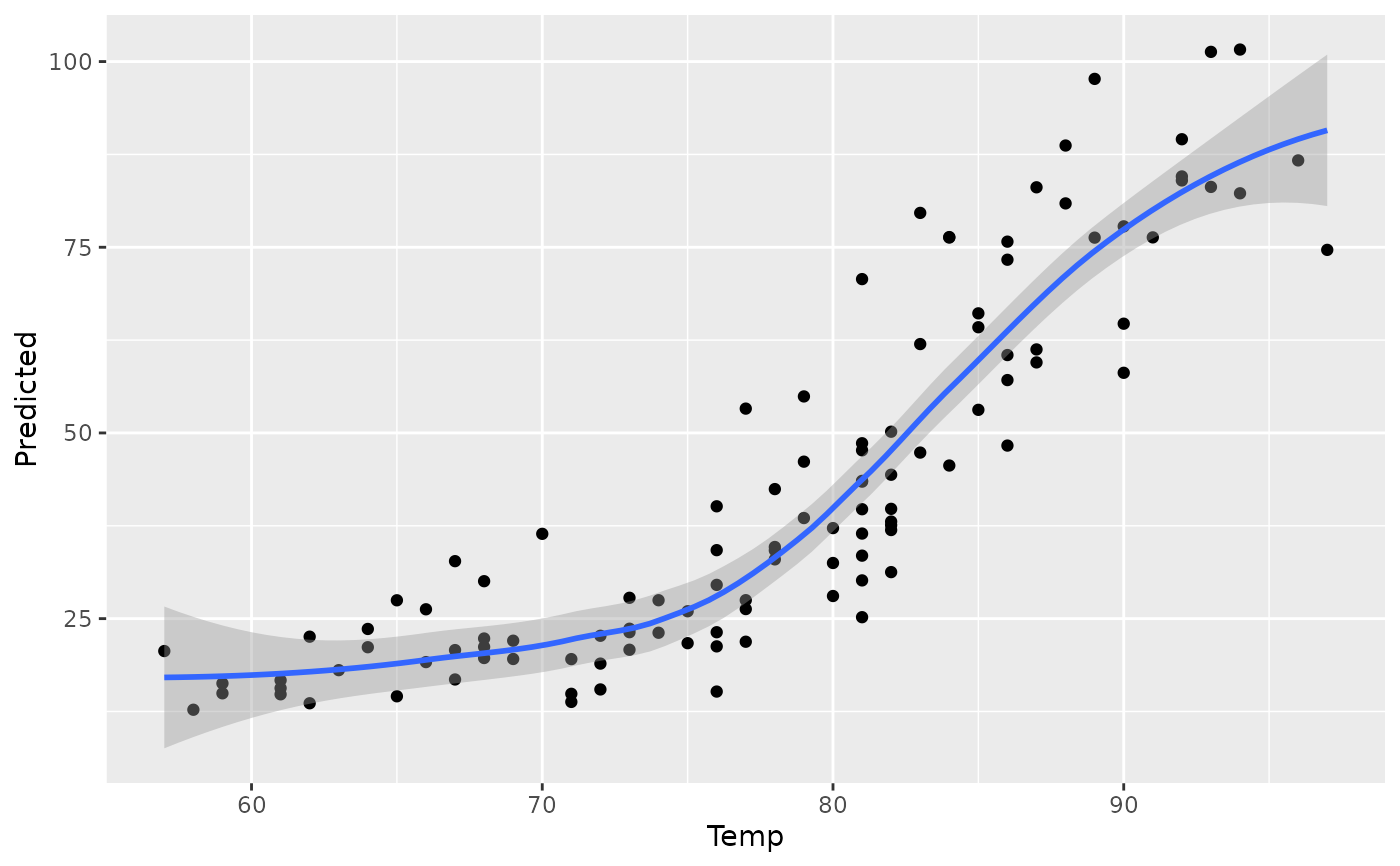
 plot(gg_dta, xvar = "Temp")
#> `geom_smooth()` using method = 'loess' and formula = 'y ~ x'
plot(gg_dta, xvar = "Temp")
#> `geom_smooth()` using method = 'loess' and formula = 'y ~ x'
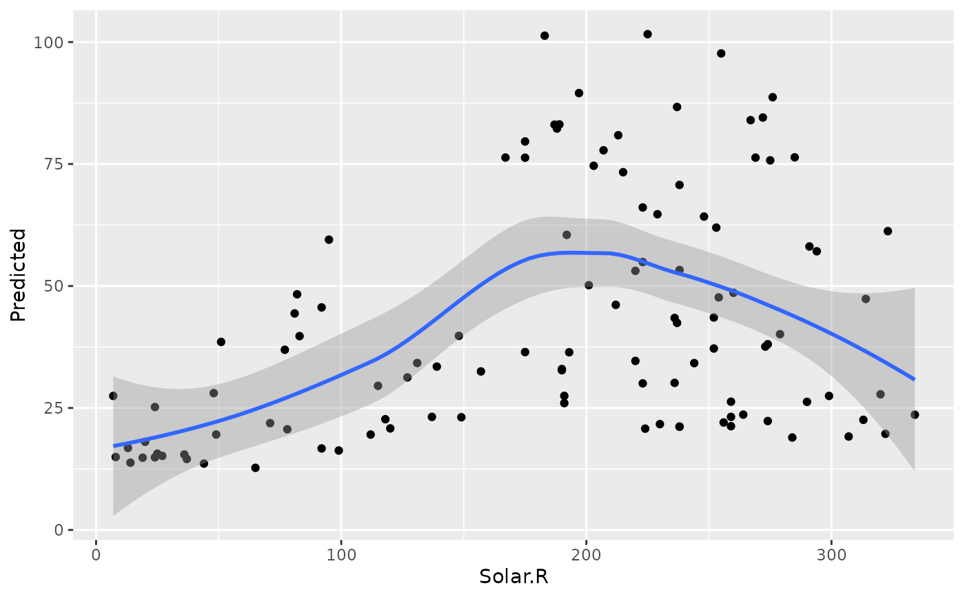
 plot(gg_dta, xvar = "Solar.R")
#> `geom_smooth()` using method = 'loess' and formula = 'y ~ x'
plot(gg_dta, xvar = "Solar.R")
#> `geom_smooth()` using method = 'loess' and formula = 'y ~ x'
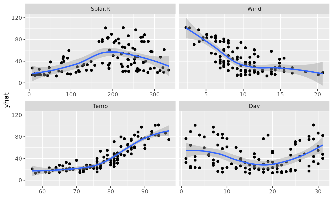
 plot(gg_dta, xvar = c("Solar.R", "Wind", "Temp", "Day"), panel = TRUE)
#> `geom_smooth()` using method = 'loess' and formula = 'y ~ x'
plot(gg_dta, xvar = c("Solar.R", "Wind", "Temp", "Day"), panel = TRUE)
#> `geom_smooth()` using method = 'loess' and formula = 'y ~ x'
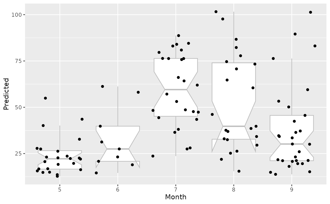
 plot(gg_dta, xvar = "Month", notch = TRUE)
#> Warning: Ignoring unknown parameters: `notch`
#> Notch went outside hinges
#> ℹ Do you want `notch = FALSE`?
#> Notch went outside hinges
#> ℹ Do you want `notch = FALSE`?
plot(gg_dta, xvar = "Month", notch = TRUE)
#> Warning: Ignoring unknown parameters: `notch`
#> Notch went outside hinges
#> ℹ Do you want `notch = FALSE`?
#> Notch went outside hinges
#> ℹ Do you want `notch = FALSE`?
 ## -------- motor trend cars data
rfsrc_mtcars <- randomForestSRC::rfsrc(mpg ~ ., data = mtcars, ntree = 50)
gg_dta <- gg_variable(rfsrc_mtcars)
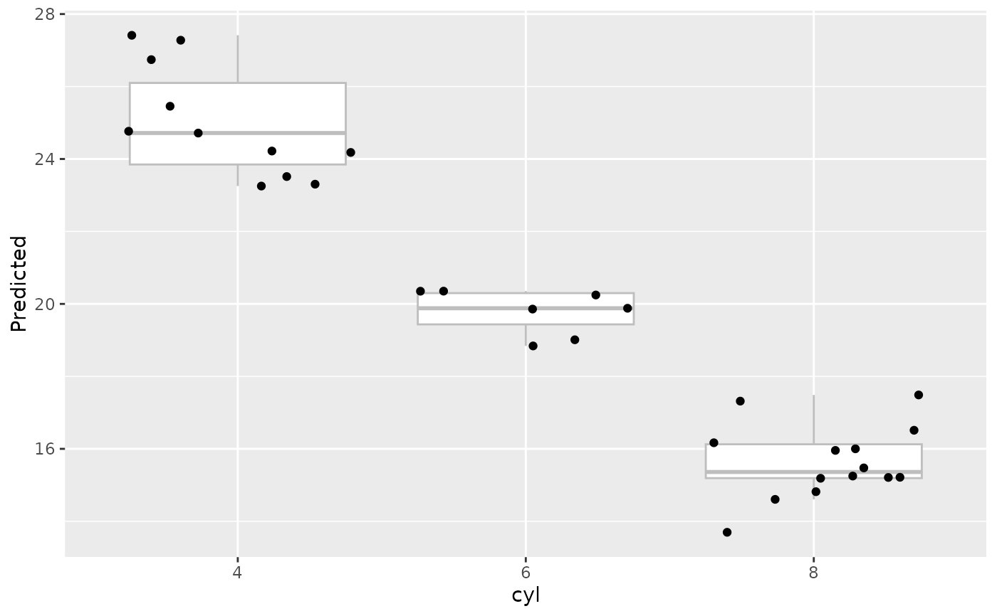
# mtcars$cyl is an ordinal variable
gg_dta$cyl <- factor(gg_dta$cyl)
gg_dta$am <- factor(gg_dta$am)
gg_dta$vs <- factor(gg_dta$vs)
gg_dta$gear <- factor(gg_dta$gear)
gg_dta$carb <- factor(gg_dta$carb)
plot(gg_dta, xvar = "cyl")
## -------- motor trend cars data
rfsrc_mtcars <- randomForestSRC::rfsrc(mpg ~ ., data = mtcars, ntree = 50)
gg_dta <- gg_variable(rfsrc_mtcars)
# mtcars$cyl is an ordinal variable
gg_dta$cyl <- factor(gg_dta$cyl)
gg_dta$am <- factor(gg_dta$am)
gg_dta$vs <- factor(gg_dta$vs)
gg_dta$gear <- factor(gg_dta$gear)
gg_dta$carb <- factor(gg_dta$carb)
plot(gg_dta, xvar = "cyl")
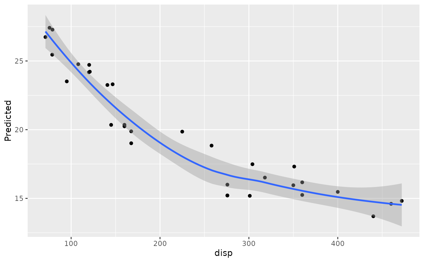
 plot(gg_dta, xvar = "disp")
#> `geom_smooth()` using method = 'loess' and formula = 'y ~ x'
plot(gg_dta, xvar = "disp")
#> `geom_smooth()` using method = 'loess' and formula = 'y ~ x'
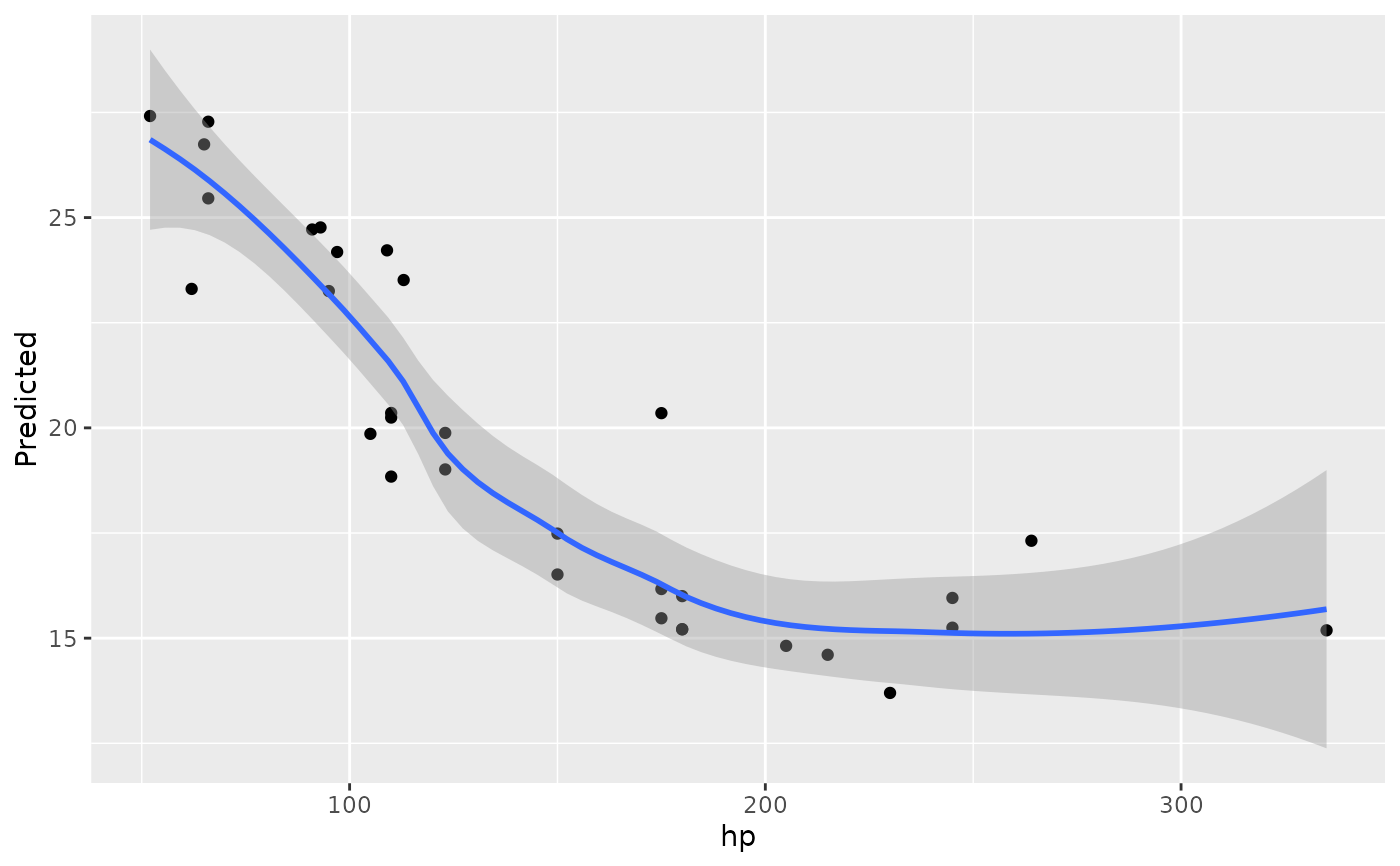
 plot(gg_dta, xvar = "hp")
#> `geom_smooth()` using method = 'loess' and formula = 'y ~ x'
plot(gg_dta, xvar = "hp")
#> `geom_smooth()` using method = 'loess' and formula = 'y ~ x'
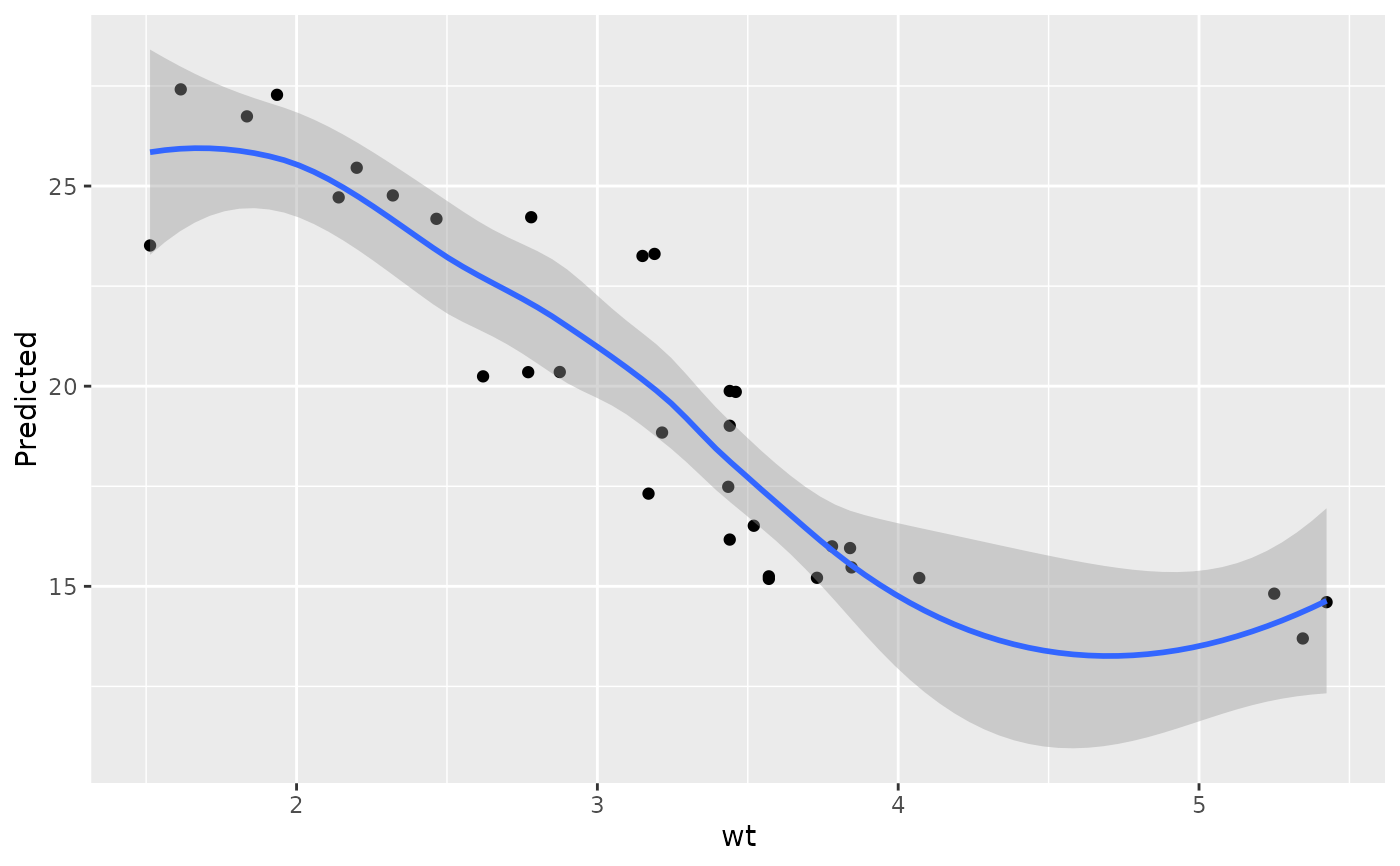
 plot(gg_dta, xvar = "wt")
#> `geom_smooth()` using method = 'loess' and formula = 'y ~ x'
plot(gg_dta, xvar = "wt")
#> `geom_smooth()` using method = 'loess' and formula = 'y ~ x'
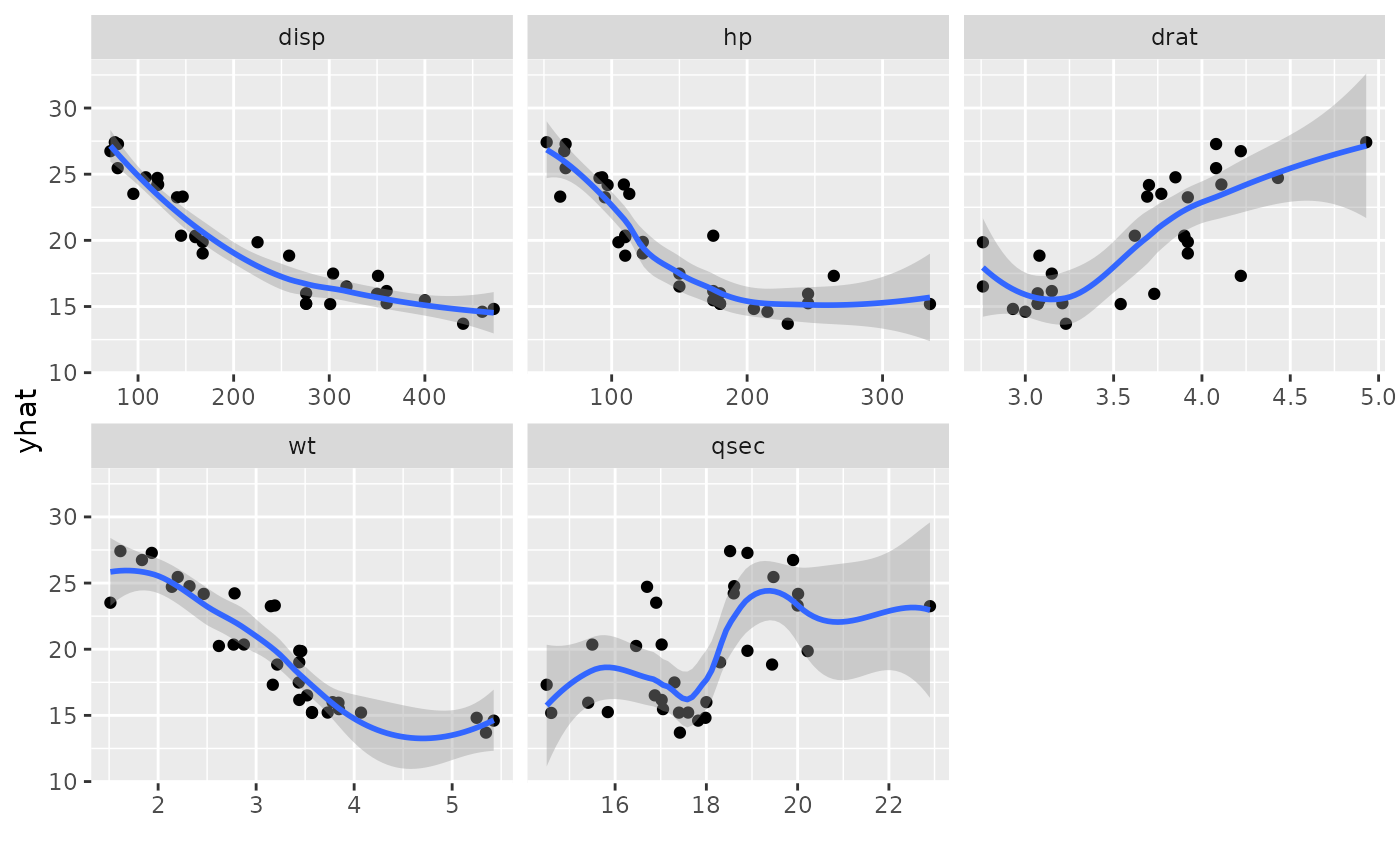
 plot(gg_dta, xvar = c("disp", "hp", "drat", "wt", "qsec"), panel = TRUE)
#> `geom_smooth()` using method = 'loess' and formula = 'y ~ x'
plot(gg_dta, xvar = c("disp", "hp", "drat", "wt", "qsec"), panel = TRUE)
#> `geom_smooth()` using method = 'loess' and formula = 'y ~ x'
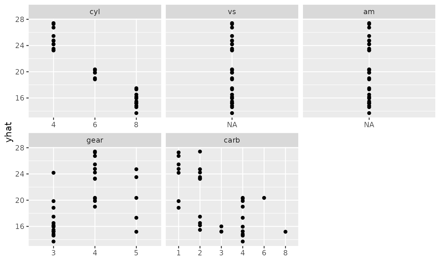
 plot(gg_dta,
xvar = c("cyl", "vs", "am", "gear", "carb"), panel = TRUE,
notch = TRUE
)
#> Warning: Ignoring unknown parameters: `notch`
#> Warning: Ignoring unknown parameters: `notch`
#> `geom_smooth()` using method = 'loess' and formula = 'y ~ x'
#> Notch went outside hinges
#> ℹ Do you want `notch = FALSE`?
#> Notch went outside hinges
#> ℹ Do you want `notch = FALSE`?
#> Notch went outside hinges
#> ℹ Do you want `notch = FALSE`?
#> Notch went outside hinges
#> ℹ Do you want `notch = FALSE`?
#> Notch went outside hinges
#> ℹ Do you want `notch = FALSE`?
#> Notch went outside hinges
#> ℹ Do you want `notch = FALSE`?
#> Notch went outside hinges
#> ℹ Do you want `notch = FALSE`?
#> Notch went outside hinges
#> ℹ Do you want `notch = FALSE`?
#> Notch went outside hinges
#> ℹ Do you want `notch = FALSE`?
#> Notch went outside hinges
#> ℹ Do you want `notch = FALSE`?
plot(gg_dta,
xvar = c("cyl", "vs", "am", "gear", "carb"), panel = TRUE,
notch = TRUE
)
#> Warning: Ignoring unknown parameters: `notch`
#> Warning: Ignoring unknown parameters: `notch`
#> `geom_smooth()` using method = 'loess' and formula = 'y ~ x'
#> Notch went outside hinges
#> ℹ Do you want `notch = FALSE`?
#> Notch went outside hinges
#> ℹ Do you want `notch = FALSE`?
#> Notch went outside hinges
#> ℹ Do you want `notch = FALSE`?
#> Notch went outside hinges
#> ℹ Do you want `notch = FALSE`?
#> Notch went outside hinges
#> ℹ Do you want `notch = FALSE`?
#> Notch went outside hinges
#> ℹ Do you want `notch = FALSE`?
#> Notch went outside hinges
#> ℹ Do you want `notch = FALSE`?
#> Notch went outside hinges
#> ℹ Do you want `notch = FALSE`?
#> Notch went outside hinges
#> ℹ Do you want `notch = FALSE`?
#> Notch went outside hinges
#> ℹ Do you want `notch = FALSE`?
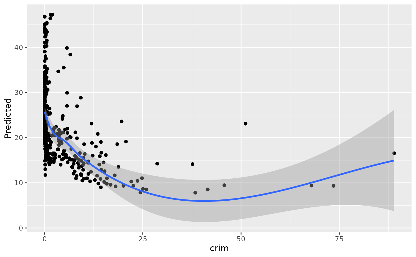
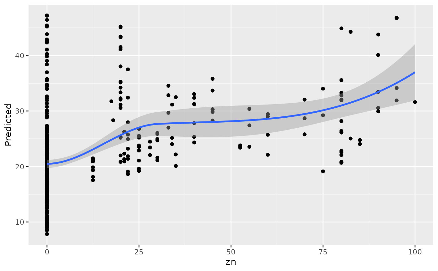
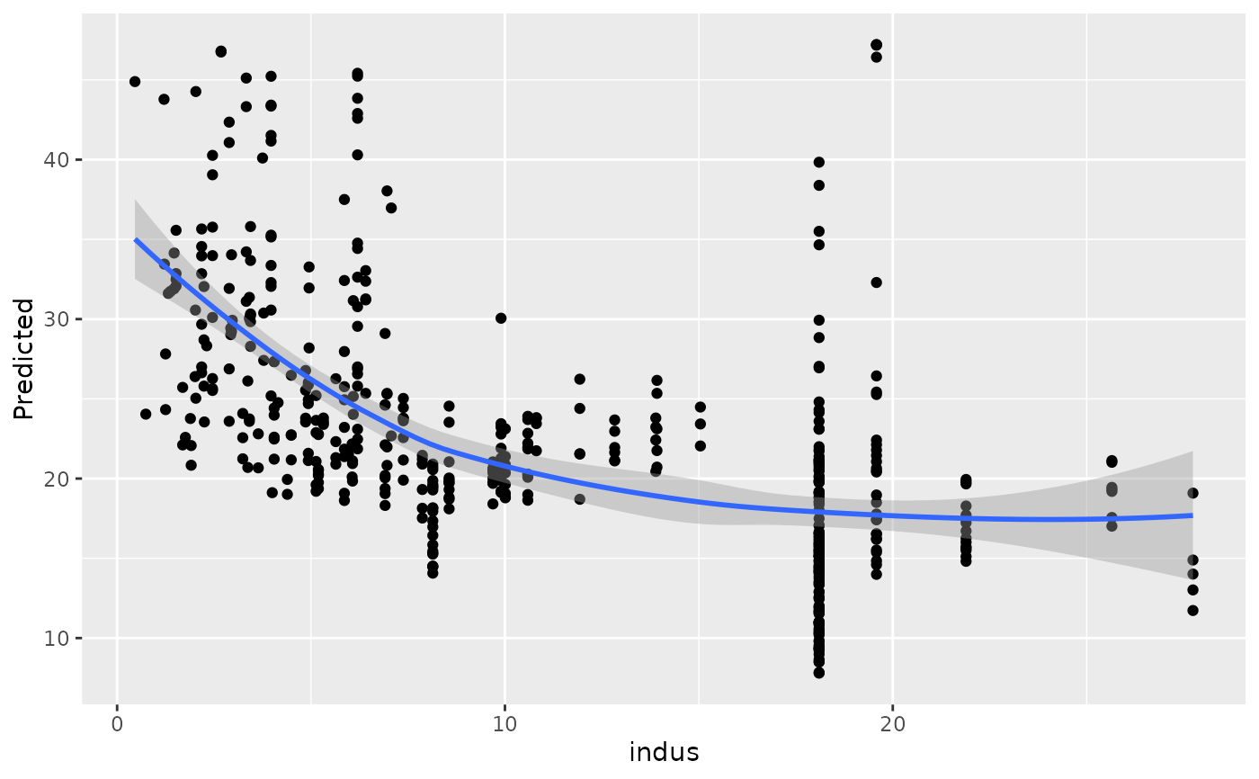
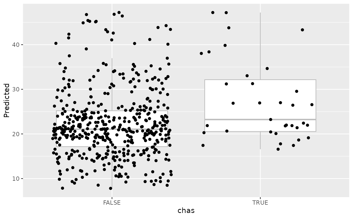
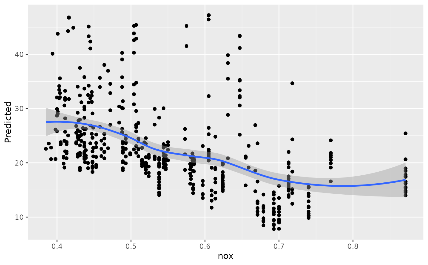
 ## -------- Boston data
if (requireNamespace("MASS", quietly = TRUE)) {
data(Boston, package = "MASS")
rf_boston <- randomForest::randomForest(medv ~ ., data = Boston)
gg_dta <- gg_variable(rf_boston)
plot(gg_dta)
plot(gg_dta, panel = TRUE)
}
#> Warning: Mismatched variable types...
#> assuming these are all factor variables.
#> Warning: Orientation is not uniquely specified when both the x and y aesthetics are
#> continuous. Picking default orientation 'x'.
#> Warning: Continuous x aesthetic
#> ℹ did you forget `aes(group = ...)`?
#> `geom_smooth()` using method = 'loess' and formula = 'y ~ x'
#> Warning: pseudoinverse used at -0.5
#> Warning: neighborhood radius 13
#> Warning: reciprocal condition number 0
#> Warning: There are other near singularities as well. 156.25
#> Warning: pseudoinverse used at -0.5
#> Warning: neighborhood radius 13
#> Warning: reciprocal condition number 0
#> Warning: There are other near singularities as well. 156.25
#> Warning: at -0.005
#> Warning: radius 2.5e-05
#> Warning: all data on boundary of neighborhood. make span bigger
#> Warning: pseudoinverse used at -0.005
#> Warning: neighborhood radius 0.005
#> Warning: reciprocal condition number 1
#> Warning: There are other near singularities as well. 1.01
#> Warning: zero-width neighborhood. make span bigger
#> Warning: Failed to fit group -1.
#> Caused by error in `predLoess()`:
#> ! NA/NaN/Inf in foreign function call (arg 5)
## -------- Boston data
if (requireNamespace("MASS", quietly = TRUE)) {
data(Boston, package = "MASS")
rf_boston <- randomForest::randomForest(medv ~ ., data = Boston)
gg_dta <- gg_variable(rf_boston)
plot(gg_dta)
plot(gg_dta, panel = TRUE)
}
#> Warning: Mismatched variable types...
#> assuming these are all factor variables.
#> Warning: Orientation is not uniquely specified when both the x and y aesthetics are
#> continuous. Picking default orientation 'x'.
#> Warning: Continuous x aesthetic
#> ℹ did you forget `aes(group = ...)`?
#> `geom_smooth()` using method = 'loess' and formula = 'y ~ x'
#> Warning: pseudoinverse used at -0.5
#> Warning: neighborhood radius 13
#> Warning: reciprocal condition number 0
#> Warning: There are other near singularities as well. 156.25
#> Warning: pseudoinverse used at -0.5
#> Warning: neighborhood radius 13
#> Warning: reciprocal condition number 0
#> Warning: There are other near singularities as well. 156.25
#> Warning: at -0.005
#> Warning: radius 2.5e-05
#> Warning: all data on boundary of neighborhood. make span bigger
#> Warning: pseudoinverse used at -0.005
#> Warning: neighborhood radius 0.005
#> Warning: reciprocal condition number 1
#> Warning: There are other near singularities as well. 1.01
#> Warning: zero-width neighborhood. make span bigger
#> Warning: Failed to fit group -1.
#> Caused by error in `predLoess()`:
#> ! NA/NaN/Inf in foreign function call (arg 5)
 ## ------------------------------------------------------------
## survival examples
## ------------------------------------------------------------
## -------- veteran data
data(veteran, package = "randomForestSRC")
rfsrc_veteran <- randomForestSRC::rfsrc(Surv(time, status) ~ ., veteran,
nsplit = 10,
ntree = 50
)
# get the 90-day survival time.
gg_dta <- gg_variable(rfsrc_veteran, time = 90)
# Generate variable dependence plots for age and diagtime
plot(gg_dta, xvar = "age")
#> `geom_smooth()` using method = 'loess' and formula = 'y ~ x'
## ------------------------------------------------------------
## survival examples
## ------------------------------------------------------------
## -------- veteran data
data(veteran, package = "randomForestSRC")
rfsrc_veteran <- randomForestSRC::rfsrc(Surv(time, status) ~ ., veteran,
nsplit = 10,
ntree = 50
)
# get the 90-day survival time.
gg_dta <- gg_variable(rfsrc_veteran, time = 90)
# Generate variable dependence plots for age and diagtime
plot(gg_dta, xvar = "age")
#> `geom_smooth()` using method = 'loess' and formula = 'y ~ x'
 plot(gg_dta, xvar = "diagtime")
#> `geom_smooth()` using method = 'loess' and formula = 'y ~ x'
plot(gg_dta, xvar = "diagtime")
#> `geom_smooth()` using method = 'loess' and formula = 'y ~ x'
 # Generate coplots
plot(gg_dta, xvar = c("age", "diagtime"), panel = TRUE, se = FALSE)
#> Warning: Ignoring unknown parameters: `se`
#> `geom_smooth()` using method = 'loess' and formula = 'y ~ x'
# Generate coplots
plot(gg_dta, xvar = c("age", "diagtime"), panel = TRUE, se = FALSE)
#> Warning: Ignoring unknown parameters: `se`
#> `geom_smooth()` using method = 'loess' and formula = 'y ~ x'
 # Compare survival at 30, 90, and 365 days simultaneously
gg_dta <- gg_variable(rfsrc_veteran, time = c(30, 90, 365))
plot(gg_dta, xvar = "age")
#> `geom_smooth()` using method = 'loess' and formula = 'y ~ x'
# Compare survival at 30, 90, and 365 days simultaneously
gg_dta <- gg_variable(rfsrc_veteran, time = c(30, 90, 365))
plot(gg_dta, xvar = "age")
#> `geom_smooth()` using method = 'loess' and formula = 'y ~ x'
 # }
# }