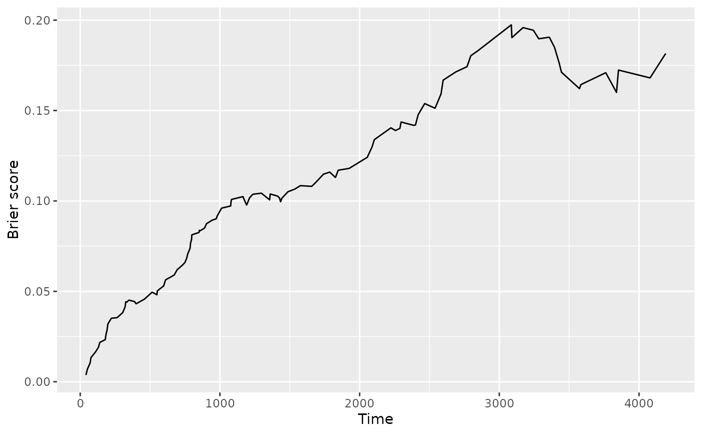
Brier score and CRPS for survival forests

The Brier score asks a familiar question of any probabilistic forecast: how far did the predicted probability sit from what actually happened? For a survival forest the forecast is the predicted survival probability at a given moment, and the "what happened" is whether the subject was still alive at that moment. The score is computed at every event time, so you get a curve rather than a single number – lower is better everywhere. A perfectly calibrated forest that predicts 0 for every subject who died and 1 for every subject who survived would score 0; a forest that predicts 0.5 for everyone scores roughly 0.25 regardless of the true outcome – that is the "uninformative" ceiling.

Usage

gg_brier(object, ...)

Arguments

object: A fitted rfsrc survival forest (object$family == "surv").
...: Currently unused; accepted for S3 dispatch compatibility.

Value

A gg_brier data.frame with columns

time: event time grid (object$time.interest).
brier: overall Brier score at each time.
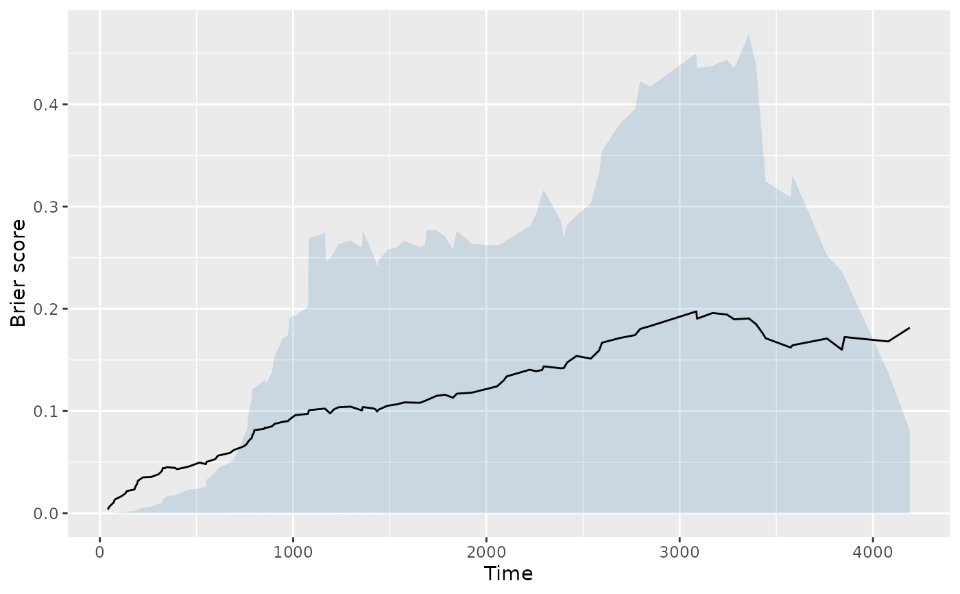
bs.q25, bs.q50, bs.q75, bs.q100: Brier score within each mortality-risk quartile (lowest to highest risk).
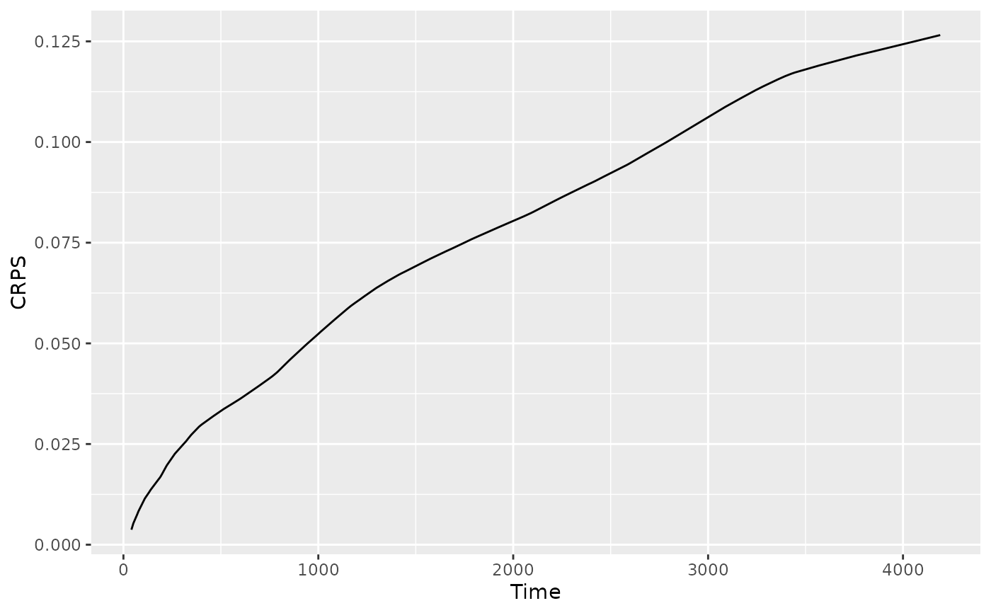
bs.lower, bs.upper: 15th and 85th percentile of per-subject Brier contributions at each time. Used by plot.gg_brier(by_quartile = TRUE) to draw an envelope around the overall curve.
crps: running CRPS (overall) at each time, normalised by elapsed time.
crps.q25, crps.q50, crps.q75, crps.q100: running CRPS within each mortality-risk quartile.
crps.lower, crps.upper: running CRPS of the 15th / 85th per-subject Brier percentile, normalised by elapsed time.

The integrated CRPS (a single scalar matching get.brier.survival()$crps) is attached as attr(., "crps_integrated").

Details

This function extracts the time-resolved Brier score for a survival forest grown with randomForestSRC, both overall and broken down by mortality-risk quartile (lowest-risk to highest-risk subjects). It also returns the continuous ranked probability score (CRPS) – the Brier score integrated over time and divided by elapsed time, a running average that summarises calibration up to each point on the time axis.

Because subjects are right-censored, a plain Brier score is biased: censored subjects contribute no outcome information yet still inflate the denominator. The score here uses inverse-probability-of-censoring weighting (IPCW), which up-weights uncensored observations to compensate. The censoring distribution is estimated either by Kaplan-Meier (cens.model = "km", the default) or by a separate censoring forest (cens.model = "rfsrc") when the censoring mechanism is itself covariate-dependent.

Internally, this wraps get.brier.survival and rebuilds the quartile decomposition and running CRPS from the returned brier.matx and mort components, following the approach in the internal plot.survival of randomForestSRC.

Note

Brier score / CRPS is randomForestSRC survival-only; there is no randomForest method.

References

Graf E., Schmoor C., Sauerbrei W., Schumacher M. (1999). Assessment and comparison of prognostic classification schemes for survival data. Statistics in Medicine, 18(17-18):2529-2545.

Gerds T.A., Schumacher M. (2006). Consistent estimation of the expected Brier score in general survival models with right-censored event times. Biometrical Journal, 48(6):1029-1040.

Examples

# \donttest{
library(survival)   # Surv() must be on the search path for rfsrc()
data(pbc, package = "randomForestSRC")
rfsrc_pbc <- randomForestSRC::rfsrc(
  Surv(days, status) ~ ., data = pbc, nsplit = 10
)
gg_dta <- gg_brier(rfsrc_pbc)
plot(gg_dta)

plot(gg_dta, type = "crps")

plot(gg_dta, envelope = TRUE)   # overall line + 15-85% envelope


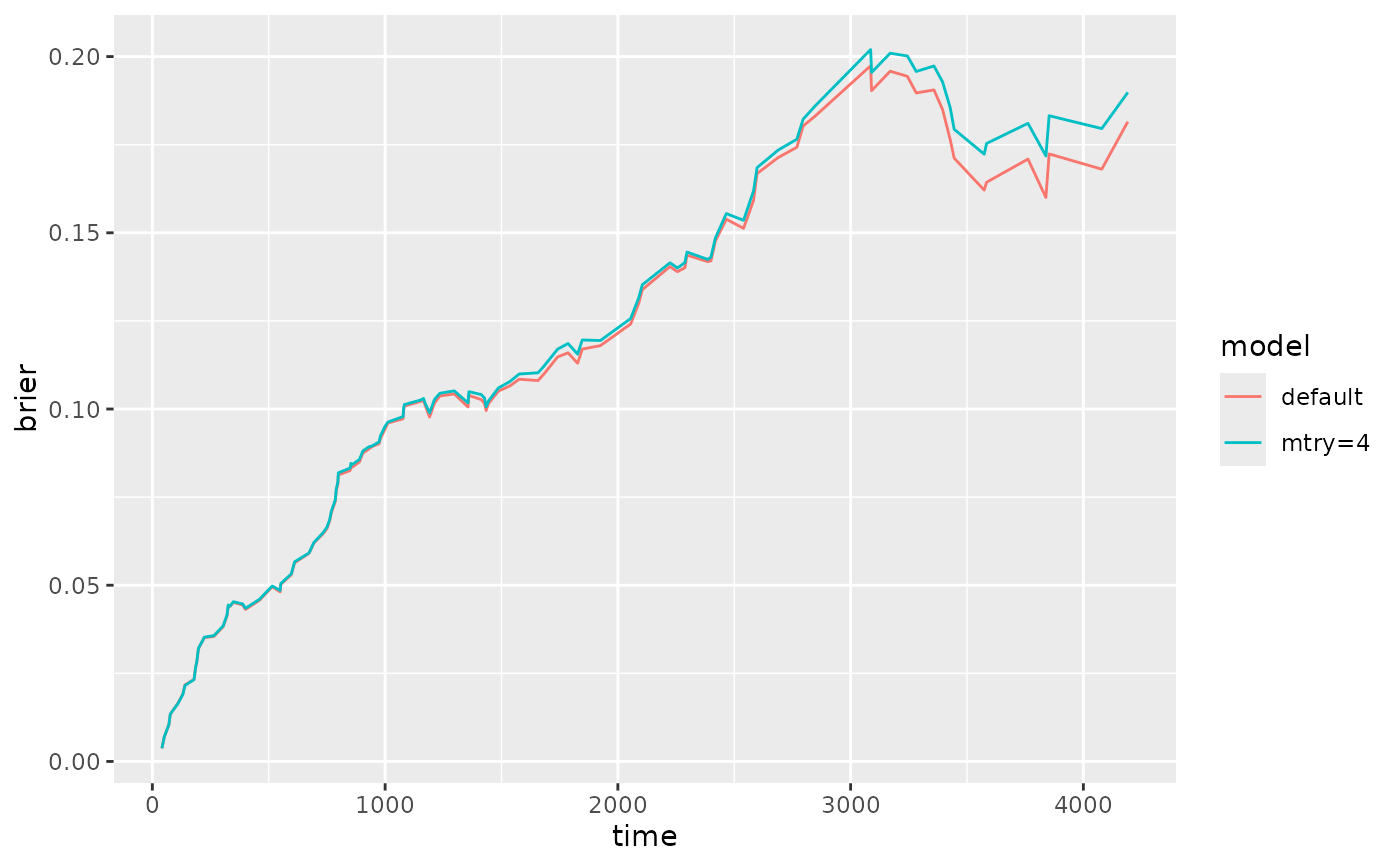
# Multi-model comparison: stack gg_brier outputs and plot with ggplot2.
rf2 <- randomForestSRC::rfsrc(
  Surv(days, status) ~ ., data = pbc, nsplit = 10, mtry = 4
)
compare_dta <- dplyr::bind_rows(
  dplyr::mutate(gg_brier(rfsrc_pbc), model = "default"),
  dplyr::mutate(gg_brier(rf2),       model = "mtry=4")
)
ggplot2::ggplot(compare_dta,
  ggplot2::aes(x = time, y = brier, colour = model)) +
  ggplot2::geom_line()

# }