Visualizes the ensemble predictions extracted by gg_rfsrc.
By default those are out-of-bag (OOB) predictions – the forest's built-in
cross-validation estimate, averaging only over the trees that left a given
observation out of their bootstrap sample.
Usage
# S3 method for class 'gg_rfsrc'
plot(x, notch = TRUE, ...)
Arguments
- x
A
gg_rfsrcobject, or a rawrfsrcobject (which will be passed throughgg_rfsrcautomatically before plotting).- notch
Logical; whether to draw notched boxplots for regression and classification forests (default
TRUE). Setnotch = FALSEto suppress notches when sample sizes are too small for reliable confidence intervals on the median.- ...
Additional arguments forwarded to the underlying
ggplot2geometry calls. Commonly useful arguments include:alphaNumeric in \([0,1]\); point/ribbon transparency. For survival plots with confidence bands the ribbon alpha is automatically halved relative to the value supplied here.
sizePoint or line size passed to
geom_jitter,geom_step, etc.
Arguments that control
gg_rfsrc(e.g.conf.int,surv_type,by) should be applied when constructing thegg_rfsrcobject before callingplot().
Value
A ggplot object. The plot appearance depends on the forest
family stored in x:
- Regression (
"regr") Jitter + notched boxplot of OOB predicted values. If a
groupcolumn is present the x-axis shows each group label; otherwise observations are collapsed to a single x-position.- Classification (
"class") Binary: jitter + notched boxplot of the predicted class probability. Multi-class: jitter plot with one panel per class (class probabilities in long form).
- Survival (
"surv") Step curves of the ensemble survival function. When
gg_rfsrcwas called withconf.int, a shaded ribbon is added. When called withby, curves are coloured by group.
Details
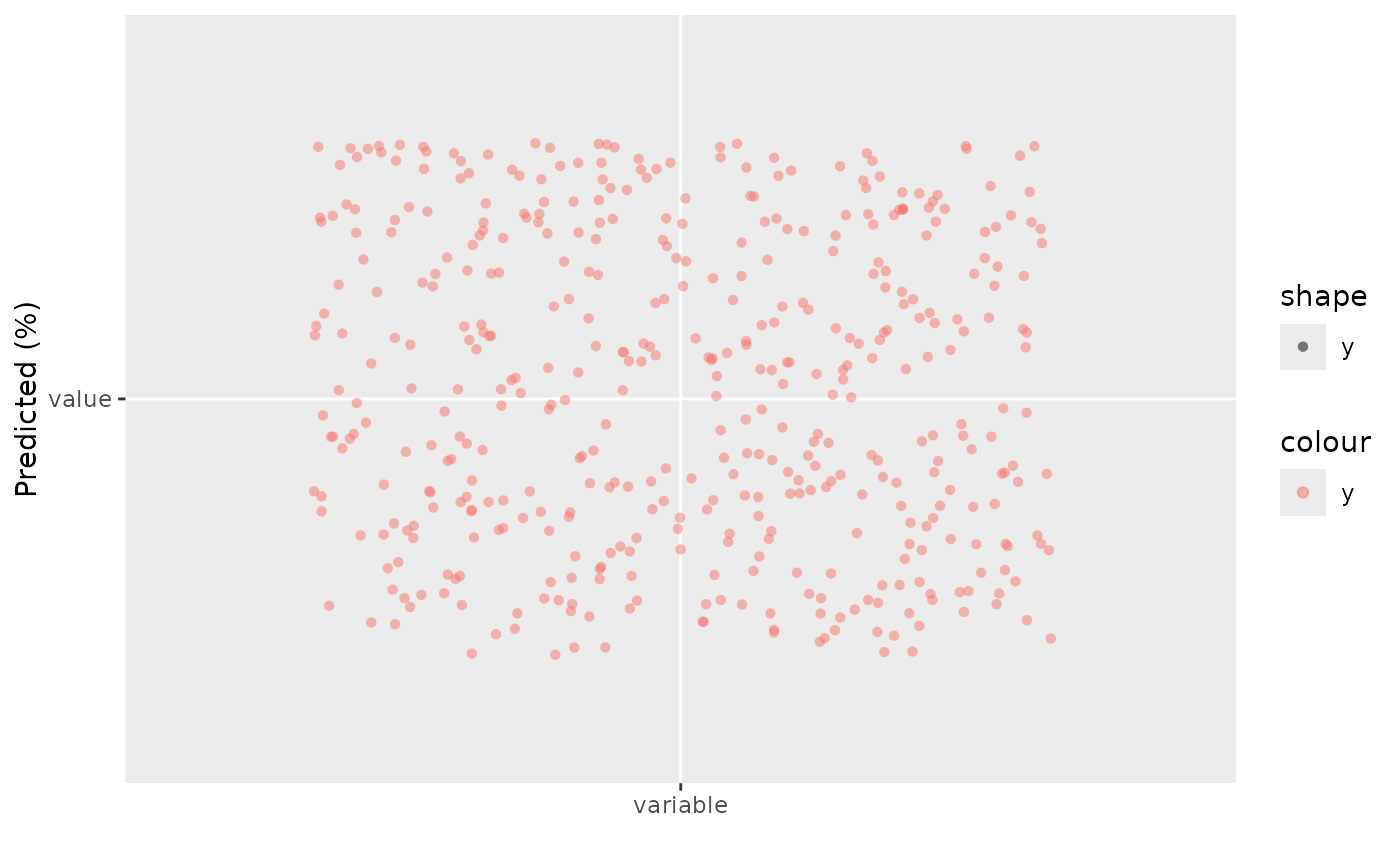
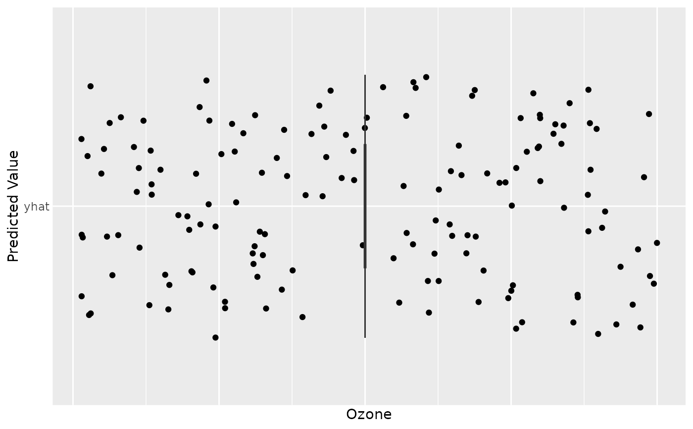
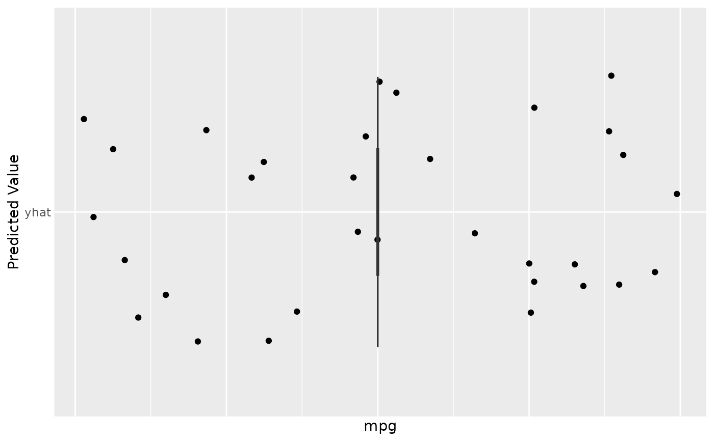
The geometry adapts to the forest family. For regression or
classification, you get a jitter-and-boxplot: every observation is a dot
placed at its OOB predicted value, coloured by observed response, with a
notched boxplot overlaid to show the central tendency and spread. For a
survival forest, each observation contributes one ensemble survival curve
(or CHF / mortality, whichever surv_type was chosen in
gg_rfsrc); the bundle of step functions shows the spread of
predicted risk across the cohort. Pass by to gg_rfsrc
beforehand to colour curves by a predictor group, or conf.int to
replace the individual curves with a mean curve and bootstrap ribbon.
References
Breiman L. (2001). Random forests, Machine Learning, 45:5-32.
Ishwaran H. and Kogalur U.B. (2007). Random survival forests for R, Rnews, 7(2):25-31.
Ishwaran H. and Kogalur U.B. randomForestSRC: Random Forests for Survival, Regression and Classification. R package version >= 3.4.0. https://cran.r-project.org/package=randomForestSRC
Examples
## ------------------------------------------------------------
## classification example
## ------------------------------------------------------------
## -------- iris data
# Build a small classification forest (ntree=50 keeps example fast)
set.seed(42)
rfsrc_iris <- randomForestSRC::rfsrc(Species ~ ., data = iris, ntree = 50)
gg_dta <- gg_rfsrc(rfsrc_iris)
plot(gg_dta)
 ## ------------------------------------------------------------
## Regression example
## ------------------------------------------------------------
## -------- air quality data
# na.action = "na.impute" handles missing Ozone / Solar.R values
set.seed(42)
rfsrc_airq <- randomForestSRC::rfsrc(Ozone ~ ., data = airquality,
na.action = "na.impute", ntree = 50)
gg_dta <- gg_rfsrc(rfsrc_airq)
plot(gg_dta)
## ------------------------------------------------------------
## Regression example
## ------------------------------------------------------------
## -------- air quality data
# na.action = "na.impute" handles missing Ozone / Solar.R values
set.seed(42)
rfsrc_airq <- randomForestSRC::rfsrc(Ozone ~ ., data = airquality,
na.action = "na.impute", ntree = 50)
gg_dta <- gg_rfsrc(rfsrc_airq)
plot(gg_dta)
 ## -------- mtcars data
set.seed(42)
rfsrc_mtcars <- randomForestSRC::rfsrc(mpg ~ ., data = mtcars, ntree = 50)
gg_dta <- gg_rfsrc(rfsrc_mtcars)
plot(gg_dta)
## -------- mtcars data
set.seed(42)
rfsrc_mtcars <- randomForestSRC::rfsrc(mpg ~ ., data = mtcars, ntree = 50)
gg_dta <- gg_rfsrc(rfsrc_mtcars)
plot(gg_dta)
 ## ------------------------------------------------------------
## Survival example
## ------------------------------------------------------------
## -------- veteran data
## randomized trial of two treatment regimens for lung cancer
data(veteran, package = "randomForestSRC")
set.seed(42)
rfsrc_veteran <- randomForestSRC::rfsrc(Surv(time, status) ~ ., data = veteran, ntree = 50)
gg_dta <- gg_rfsrc(rfsrc_veteran)
plot(gg_dta)
## ------------------------------------------------------------
## Survival example
## ------------------------------------------------------------
## -------- veteran data
## randomized trial of two treatment regimens for lung cancer
data(veteran, package = "randomForestSRC")
set.seed(42)
rfsrc_veteran <- randomForestSRC::rfsrc(Surv(time, status) ~ ., data = veteran, ntree = 50)
gg_dta <- gg_rfsrc(rfsrc_veteran)
plot(gg_dta)
 # With 95% pointwise bootstrap confidence bands
gg_dta <- gg_rfsrc(rfsrc_veteran, conf.int = .95)
plot(gg_dta)
# With 95% pointwise bootstrap confidence bands
gg_dta <- gg_rfsrc(rfsrc_veteran, conf.int = .95)
plot(gg_dta)
 # Stratified by treatment arm
gg_dta <- gg_rfsrc(rfsrc_veteran, by = "trt")
plot(gg_dta)
# Stratified by treatment arm
gg_dta <- gg_rfsrc(rfsrc_veteran, by = "trt")
plot(gg_dta)
 ## -------- pbc data (larger dataset -- skipped on CRAN)
# \donttest{
data(pbc, package = "randomForestSRC")
# For whatever reason, the age variable is in days; convert to years
for (ind in seq_len(dim(pbc)[2])) {
if (!is.factor(pbc[, ind])) {
if (length(unique(pbc[which(!is.na(pbc[, ind])), ind])) <= 2) {
if (sum(range(pbc[, ind], na.rm = TRUE) == c(0, 1)) == 2) {
pbc[, ind] <- as.logical(pbc[, ind])
}
}
} else {
if (length(unique(pbc[which(!is.na(pbc[, ind])), ind])) <= 2) {
if (sum(sort(unique(pbc[, ind])) == c(0, 1)) == 2) {
pbc[, ind] <- as.logical(pbc[, ind])
}
if (sum(sort(unique(pbc[, ind])) == c(FALSE, TRUE)) == 2) {
pbc[, ind] <- as.logical(pbc[, ind])
}
}
}
if (!is.logical(pbc[, ind]) &
length(unique(pbc[which(!is.na(pbc[, ind])), ind])) <= 5) {
pbc[, ind] <- factor(pbc[, ind])
}
}
# Convert age from days to years
pbc$age <- pbc$age / 364.24
pbc$years <- pbc$days / 364.24
pbc <- pbc[, -which(colnames(pbc) == "days")]
pbc$treatment <- as.numeric(pbc$treatment)
pbc$treatment[which(pbc$treatment == 1)] <- "DPCA"
pbc$treatment[which(pbc$treatment == 2)] <- "placebo"
pbc$treatment <- factor(pbc$treatment)
# Remove test-set patients (those with no assigned treatment)
dta_train <- pbc[-which(is.na(pbc$treatment)), ]
set.seed(42)
rfsrc_pbc <- randomForestSRC::rfsrc(
Surv(years, status) ~ .,
dta_train,
nsplit = 10,
na.action = "na.impute",
forest = TRUE,
importance = TRUE,
save.memory = TRUE
)
gg_dta <- gg_rfsrc(rfsrc_pbc)
plot(gg_dta)
## -------- pbc data (larger dataset -- skipped on CRAN)
# \donttest{
data(pbc, package = "randomForestSRC")
# For whatever reason, the age variable is in days; convert to years
for (ind in seq_len(dim(pbc)[2])) {
if (!is.factor(pbc[, ind])) {
if (length(unique(pbc[which(!is.na(pbc[, ind])), ind])) <= 2) {
if (sum(range(pbc[, ind], na.rm = TRUE) == c(0, 1)) == 2) {
pbc[, ind] <- as.logical(pbc[, ind])
}
}
} else {
if (length(unique(pbc[which(!is.na(pbc[, ind])), ind])) <= 2) {
if (sum(sort(unique(pbc[, ind])) == c(0, 1)) == 2) {
pbc[, ind] <- as.logical(pbc[, ind])
}
if (sum(sort(unique(pbc[, ind])) == c(FALSE, TRUE)) == 2) {
pbc[, ind] <- as.logical(pbc[, ind])
}
}
}
if (!is.logical(pbc[, ind]) &
length(unique(pbc[which(!is.na(pbc[, ind])), ind])) <= 5) {
pbc[, ind] <- factor(pbc[, ind])
}
}
# Convert age from days to years
pbc$age <- pbc$age / 364.24
pbc$years <- pbc$days / 364.24
pbc <- pbc[, -which(colnames(pbc) == "days")]
pbc$treatment <- as.numeric(pbc$treatment)
pbc$treatment[which(pbc$treatment == 1)] <- "DPCA"
pbc$treatment[which(pbc$treatment == 2)] <- "placebo"
pbc$treatment <- factor(pbc$treatment)
# Remove test-set patients (those with no assigned treatment)
dta_train <- pbc[-which(is.na(pbc$treatment)), ]
set.seed(42)
rfsrc_pbc <- randomForestSRC::rfsrc(
Surv(years, status) ~ .,
dta_train,
nsplit = 10,
na.action = "na.impute",
forest = TRUE,
importance = TRUE,
save.memory = TRUE
)
gg_dta <- gg_rfsrc(rfsrc_pbc)
plot(gg_dta)
 gg_dta <- gg_rfsrc(rfsrc_pbc, conf.int = .95)
plot(gg_dta)
gg_dta <- gg_rfsrc(rfsrc_pbc, conf.int = .95)
plot(gg_dta)
 gg_dta <- gg_rfsrc(rfsrc_pbc, by = "treatment")
plot(gg_dta)
gg_dta <- gg_rfsrc(rfsrc_pbc, by = "treatment")
plot(gg_dta)
 # }
# }