Prepare longitudinal participation counts data for plotting

Validates a pre-aggregated long-format counts data frame and returns an hv_longitudinal object. Call plot.hv_longitudinal on the result with type = "plot" for the grouped bar chart or type = "table" for the numeric text-table panel. Compose both panels with patchwork.

Usage

hv_longitudinal(
  data,
  x_col = "time_label",
  count_col = "count",
  group_col = "series"
)

Arguments

data

Long-format data frame; one row per series per time point. See sample_longitudinal_counts_data.

x_col

Name of the discrete time-label column. Default "time_label".

count_col

Name of the numeric count column. Default "count".

group_col

Name of the series grouping column. Default "series".

Value

An object of class c("hv_longitudinal", "hv_data"):

$data

The validated input data frame.

$meta

Named list: x_col, count_col, group_col, n_timepoints, n_groups, n_obs.

$tables

Empty list.

See also

plot.hv_longitudinal, sample_longitudinal_counts_data

Examples

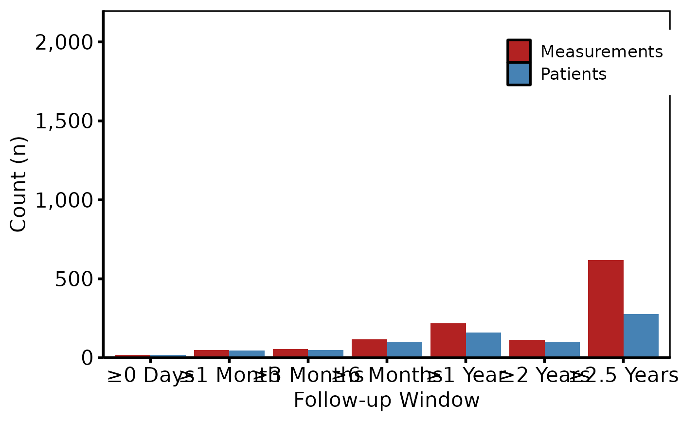
dta <- sample_longitudinal_counts_data(n_patients = 300, seed = 42L)

# 1. Build data object
lc <- hv_longitudinal(dta)
lc  # prints group/time-point counts
#> <hv_longitudinal>
#>   Time points : 7
#>   Groups      : 2  (14 rows)
#>   x / count / group : time_label / count / series

# 2. Bare plot -- undecorated ggplot returned by plot.hv_longitudinal
library(ggplot2)
p <- plot(lc, type = "plot")

# 3. Decorate: fill palette, y-axis scale, labels, theme
p +
  scale_fill_manual(
    values = c(Patients = "steelblue", Measurements = "firebrick"),
    name   = NULL
  ) +
  scale_y_continuous(labels = scales::comma,
                     breaks = seq(0, 2000, 500),
                     expand = c(0, 0)) +
  coord_cartesian(ylim = c(0, 2200)) +
  labs(x = "Follow-up Window", y = "Count (n)") +
  hv_theme("poster") +
  theme(legend.position = c(0.85, 0.85))