Prepare mirror-histogram data for plotting

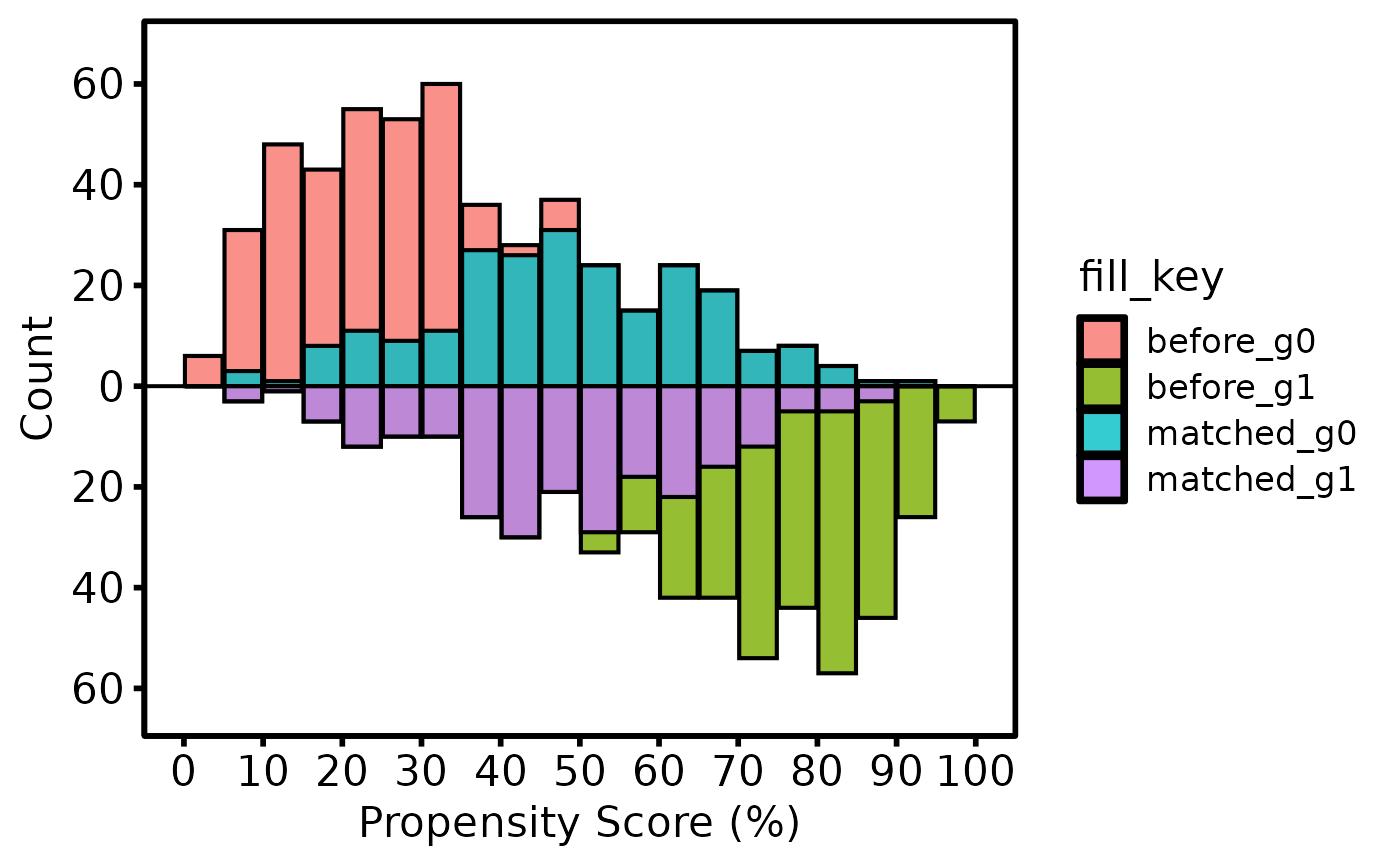
Validates and assembles propensity-score distributions for a mirrored histogram comparing a treated group (bars above the axis) and a control group (bars below the axis), with optional matched and unmatched shading. Returns an hv_mirror_hist object; call plot.hv_mirror_hist on the result to obtain a bare ggplot2 object.

Usage

hv_mirror_hist(
  data,
  score_col = "prob_t",
  group_col = "tavr",
  match_col = "match",
  group_levels = c(0, 1),
  group_labels = c("SAVR", "TF-TAVR"),
  matched_value = 1,
  score_multiplier = HVTI_SCORE_DEFAULT_MULTIPLIER,
  binwidth = 5,
  weight_col = NULL
)

Arguments

data

A data frame with one row per patient.

score_col

Name of the propensity-score column (0–1 scale before multiplier is applied). Default "prob_t".

group_col

Name of the binary group-indicator column. Default "tavr".

match_col

Name of the binary match-indicator column (1 = matched). Default "match".

group_levels

Length-2 vector of the two values in group_col (control first, treated second). Default c(0, 1).

group_labels

Length-2 character vector of display labels corresponding to group_levels. Default c("SAVR", "TF-TAVR").

matched_value

Value in match_col that flags a matched patient. Default 1.

score_multiplier

Scalar applied to score_col to convert to the 0–100 display scale. Default 100.

binwidth

Histogram bin width on the 0–100 scale. Default 5.

weight_col

Optional name of an IPTW weight column. When supplied, bar heights reflect weighted counts instead of raw counts.

Value

An object of class c("hv_mirror_hist", "hv_data"); call plot() on the result to render the figure — see plot.hv_mirror_hist. The list contains:

$data

Tidy data frame of histogram bar coordinates for plot.hv_mirror_hist.

$meta

Named list: score_col, group_col, match_col, group_labels, binwidth, lower, upper, y_breaks, n_obs, n_dropped.

$tables

Named list with two elements:

diagnostics

A named list of diagnostic summaries. Always contains n_input, n_analyzed, n_dropped_missing_or_other_group, group_counts_before (table), score_summary_before (by object), and smd_before (numeric SMD). In binary-match mode, additionally contains group_counts_matched, matched_rate_by_group, score_summary_matched, and smd_matched. In weighted IPTW mode, additionally contains effective_n_by_group and smd_weighted.

working

The per-patient data frame after score rescaling and complete-case filtering, used for custom downstream diagnostics.

See also

plot.hv_mirror_hist to render as a ggplot2 figure, hv_theme for the publication theme, sample_mirror_histogram_data for example data.

Other Propensity Score & Matching: plot.hv_mirror_hist()

Examples

dta <- sample_mirror_histogram_data(n = 500, separation = 1.5)

# 1. Build data object
mh <- hv_mirror_hist(dta)
#> mirror_histogram diagnostics: n=1000  dropped=0  [see $tables$diagnostics]
mh                    # print diagnostics summary
#> <hv_mirror_hist>
#>   Groups      : SAVR (control) vs TF-TAVR (treated)
#>   Score col   : prob_t
#>   Match col   : match
#>   N obs       : 1000  (dropped: 0)
#>   Bin width   : 5
#>   Y range     : [-63, 66]
#>   $tables     : diagnostics, working
mh$tables$diagnostics # full diagnostics list
#> $n_input
#> [1] 1000
#> 
#> $n_analyzed
#> [1] 1000
#> 
#> $n_dropped_missing_or_other_group
#> [1] 0
#> 
#> $group_counts_before
#> 
#>   0   1 
#> 500 500 
#> 
#> $score_summary_before
#> working$group: 0
#>    Min. 1st Qu.  Median    Mean 3rd Qu.    Max. 
#>   2.313  19.614  31.260  34.205  47.144  90.167 
#> ------------------------------------------------------------ 
#> working$group: 1
#>    Min. 1st Qu.  Median    Mean 3rd Qu.    Max. 
#>   6.775  51.385  67.926  64.596  81.283  98.587 
#> 
#> $smd_before
#> [1] 1.565275
#> 
#> $group_counts_matched
#> 
#>   0   1 
#> 230 230 
#> 
#> $matched_rate_by_group
#>    0    1 
#> 0.46 0.46 
#> 
#> $score_summary_matched
#> working$group[matched_idx]: 0
#>    Min. 1st Qu.  Median    Mean 3rd Qu.    Max. 
#>   6.904  38.323  48.337  48.565  61.152  90.167 
#> ------------------------------------------------------------ 
#> working$group[matched_idx]: 1
#>    Min. 1st Qu.  Median    Mean 3rd Qu.    Max. 
#>   6.775  38.321  48.425  48.872  61.136  89.236 
#> 
#> $smd_matched
#> [1] 0.01837958
#> 

# 2. Bare plot -- undecorated ggplot returned by plot.hv_mirror_hist
p <- plot(mh)

# 3. Decorate: axis labels and theme
p +
  ggplot2::labs(x = "Propensity Score (%)", y = "Count") +
  hv_theme("poster")