dta <- sample_ps_data(n = 500, seed = 42)
head(dta)
#>   id tavr      age female       ef diabetes hypertension    prob_t match
#> 1  1    0 88.96767      1 35.91940        0            1 0.1072885     0
#> 2  2    0 73.48241      0 32.50216        1            0 0.2258719     0
#> 3  3    0 80.90503      1 48.59300        0            1 0.3249308     0
#> 4  4    0 83.06290      0 53.74726        0            1 0.2872581     0
#> 5  5    0 81.23415      0 29.22222        1            1 0.0920883     0
#> 6 6 0 77.15100 0 54.90524 0 0 0.4674866 01 Overview
hvtiRpropensity provides propensity score methods for cardiac surgery comparative-effectiveness research. It ports the balancing logic from six SAS templates into a tidy R API whose outputs feed hvtiPlotR. The six templates ship with the package, in system.file("sas-templates", package = "hvtiRpropensity").
The package covers the full workflow from raw covariates to sensitivity analysis:
-
Estimate a balancing score:
ps_logistic(),ps_forest(),ps_ordinal(),ps_nominal(),bs_continuous(),bs_count(). -
Balance treatment groups:
ps_match()(nearest-neighbour matching) orps_weight()(IPTW). -
Diagnose balance and support: the SMD tables, group counts and effective sample sizes in
$tables,ps_stddiff()andps_stddiff_perm(), andps_support()for the common-support rules. -
Estimate the effect:
ps_mw_var()for a matching-weight difference in means,ps_rmst()for restricted mean survival. -
Check the assumptions:
sa_overlap()andsa_trim_sweep()for positivity and overlap,sa_rosenbaum()andsa_evalue()for unmeasured confounding.
All score, balance, sensitivity, fit, and validation objects share a common ps_data S3 base class with four slots: $data carries patient-level outputs, $meta records the declared contract and row accounting, $tables carries inference and diagnostics, and $models retains every fitted model used to create the result.
2 Sample data
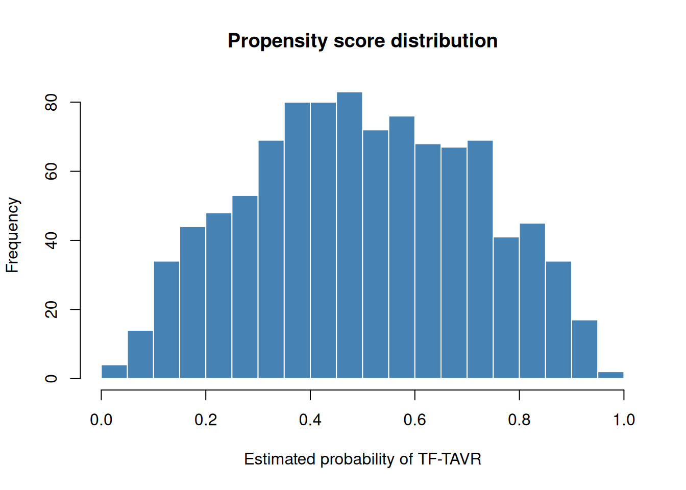
sample_ps_data() generates a synthetic cardiac-surgery dataset that mimics a typical SAS export: two treatment arms (SAVR / TF-TAVR), several continuous and binary covariates, a fitted propensity score (prob_t), and a match indicator initialised to 0.
The two treatment groups differ on all covariates (younger patients with higher ejection fraction were more likely to receive TF-TAVR), so the raw SMDs are non-trivial and the propensity scores have good overlap.
hist(
  dta$prob_t,
  breaks = 30,
  main   = "Propensity score distribution",
  xlab   = "Estimated probability of TF-TAVR",
  col    = "steelblue",
  border = "white"
)
3 Outcome-model bundles
fit_logistic() fits binary, proportional-odds ordinal, and generalized-logit nominal outcome models. The complete outcome levels and the event or reference level are required. This makes the scientific contrast independent of factor storage order.
outcome_model <- fit_logistic(
  tavr ~ age + female + ef + diabetes + hypertension,
  data = dta,
  family = "binary",
  outcome_levels = c(0, 1),
  event_level = 1
)
outcome_model$tables$estimates
#>           term    estimate   std.error statistic  df      p.value    conf.low
#> 1  (Intercept)  4.33969066 0.794459051  5.462447 Inf 4.696151e-08  2.78257953
#> 2          age -0.09351411 0.009427068 -9.919745 Inf 3.416280e-23 -0.11199082
#> 3       female  0.23341073 0.141967346  1.644116 Inf 1.001523e-01 -0.04484016
#> 4           ef  0.04999120 0.006963766  7.178759 Inf 7.034695e-13  0.03634247
#> 5     diabetes -0.32463972 0.158007358 -2.054586 Inf 3.991900e-02 -0.63432845
#> 6 hypertension -0.16776550 0.143950649 -1.165438 Inf 2.438419e-01 -0.44990358
#>     conf.high odds_ratio pooled
#> 1  5.89680179 76.6838145  FALSE
#> 2 -0.07503740  0.9107252  FALSE
#> 3  0.51166161  1.2629001  FALSE
#> 4  0.06363993  1.0512618  FALSE
#> 5 -0.01495099  0.7227877  FALSE
#> 6  0.11437259  0.8455521  FALSE
outcome_model$tables$fit_status
#>   imputation converged n_input n_analyzed n_excluded
#> 1          1      TRUE    1000       1000          0
Every bundle records bundle_version = 1L, the formula, required predictors, declared outcome levels, package versions, analysis counts, all model objects, and four common inference tables:
| table | schema |
|---|---|
estimates |
term, estimate, std.error, statistic, df, p.value, conf.low, conf.high, odds_ratio (rate_ratio for the log-link count family), pooled
|
covariance |
named coefficient covariance matrix |
by_imputation |
imputation, term, estimate, std.error
|
fit_status |
imputation, converged, n_input, n_analyzed, n_excluded
|
For stacked long-form imputations, the same model is fit independently within each imputation. Predictions are averaged patient by patient, matching the legacy PROC SUMMARY mean= workflow, while coefficient inference and covariance use Rubin’s rules. These answer different questions and are stored separately. A missing patient, changed outcome or categorical predictor level, aliased term, failed fit, or unusable covariance stops pooling.
dta_mi <- do.call(rbind, lapply(1:3, function(imputation) {
  partition <- dta
  partition$age <- partition$age + (imputation - 2) / 10
  partition$imputation <- imputation
  partition
}))

outcome_model_mi <- fit_logistic(
  tavr ~ age + female + ef + diabetes + hypertension,
  data = dta_mi,
  family = "binary",
  id_col = "id",
  imputation_col = "imputation",
  outcome_levels = c(0, 1),
  event_level = 1
)
outcome_model_mi$tables$estimates
#>           term    estimate   std.error statistic      df      p.value
#> 1  (Intercept)  4.33969066 0.794532803  5.461940 991.806 5.954560e-08
#> 2          age -0.09351411 0.009427068 -9.919745 992.006 3.535981e-22
#> 3       female  0.23341073 0.141967346  1.644116 992.006 1.004692e-01
#> 4           ef  0.04999120 0.006963766  7.178759 992.006 1.377630e-12
#> 5     diabetes -0.32463972 0.158007358 -2.054586 992.006 4.018051e-02
#> 6 hypertension -0.16776550 0.143950649 -1.165438 992.006 2.441221e-01
#>      conf.low   conf.high odds_ratio pooled
#> 1  2.78053228  5.89884904 76.6838145   TRUE
#> 2 -0.11201339 -0.07501482  0.9107252   TRUE
#> 3 -0.04518007  0.51200152  1.2629001   TRUE
#> 4  0.03632580  0.06365661  1.0512618   TRUE
#> 5 -0.63470676 -0.01457268  0.7227877   TRUE
#> 6 -0.45024824  0.11471725  0.8455521   TRUE
outcome_model_mi$tables$fit_status
#>   imputation converged n_input n_analyzed n_excluded
#> 1          1      TRUE    1000       1000          0
#> 2          2      TRUE    1000       1000          0
#> 3          3      TRUE    1000       1000          0
validate_logistic() scores a validation cohort from a saved binary bundle without refitting and without modifying the source object. It returns equal-frequency calibration groups and a performance row containing observed and expected event counts, O:E ratio, AUC, and Brier score. The first interface is intentionally binary only.
validation <- validate_logistic(outcome_model, dta, groups = 10L)
validation$tables$performance
#>      n observed expected oe_ratio     auc     brier
#> 1 1000      500      500        1 0.74406 0.2044163
4 Propensity score estimation
4.1 Binary treatment: ps_logistic()
In practice a propensity score is estimated from covariates before matching or weighting. ps_logistic() fits stats::glm(..., family = binomial()) and appends several columns that mirror the original SAS template output:
| R column | SAS equivalent | Description |
|---|---|---|
prob_t |
_p_ / _propen_
|
Propensity score (probability of treatment) |
logit_t |
_logit_ |
Log-odds: log(p / (1 - p))
|
mt_wt |
mt_wt |
Matching weight min(p, 1-p) / (p·trt + (1-p)·(1-trt))
|
quintile |
quintile |
Rank-based quintile (1–5) |
decile |
decile |
Rank-based decile (1–10) |
dta_ps <- sample_ps_data(n = 500, seed = 42)
dta_ps$prob_t <- NULL
obj_ps <- ps_logistic(
  tavr ~ age + female + ef + diabetes + hypertension,
  data = dta_ps
)
print(obj_ps)
#> <ps_logistic>
#>   N total     : 1000
#>   Treatment   : tavr
#>   PS column   : prob_t
#>   Weight col  : mt_wt
#>   Method      : logistic
#>   Tables      : smd, group_counts, estimates, covariance, by_imputation, fit_status
The scored dataset can be passed directly to ps_match() or ps_weight().
head(obj_ps$data[, c("id", "tavr", "prob_t", "logit_t", "mt_wt",
                      "quintile", "decile")])
#>   id tavr    prob_t    logit_t     mt_wt quintile decile
#> 1  1    0 0.1072885 -2.1187424 0.1201827        1      1
#> 2  2    0 0.2258719 -1.2317694 0.2917758        1      2
#> 3  3    0 0.3249308 -0.7312031 0.4813295        2      3
#> 4  4    0 0.2872581 -0.9087381 0.4030325        1      2
#> 5  5    0 0.0920883 -2.2883993 0.1014287        1      1
#> 6 6 0 0.4674866 -0.1302375 0.8778869 3 54.2 Multiply-imputed data
The SAS template fits the model separately on each imputed dataset (PROC LOGISTIC ... BY _IMPUTATION_) and averages predicted probabilities with PROC SUMMARY mean=. Pass a stacked long-format MI data frame and set imputation_col to replicate this.
dta_base <- sample_ps_data(n = 300, seed = 10)
dta_base$prob_t <- NULL

# Simulate two imputed datasets stacked with an imputation index column
dta_mi <- rbind(cbind(dta_base, imp = 1L),
                cbind(dta_base, imp = 2L))

obj_mi <- ps_logistic(
  tavr ~ age + female + ef + diabetes + hypertension,
  data           = dta_mi,
  imputation_col = "imp",
  id_col         = "id"
)
print(obj_mi)
#> <ps_logistic>
#>   N total     : 600
#>   Treatment   : tavr
#>   PS column   : prob_t
#>   Weight col  : mt_wt
#>   Method      : logistic-MI (2 imputations)
#>   Tables      : smd, group_counts, estimates, covariance, by_imputation, fit_status

# Per-patient PS is averaged across imputations, matching PROC SUMMARY mean=
summary(obj_mi$data$prob_t)
#>    Min. 1st Qu.  Median    Mean 3rd Qu.    Max.
#> 0.02227 0.30987 0.48499 0.50000 0.68398 0.94193
4.3 Random-forest score: ps_forest()
When you would rather not commit to a main-effects logistic model, ps_forest() grows a classification forest with randomForestSRC and scores each patient out-of-bag, using only the trees that did not see that patient. It appends the same prob_t, logit_t, mt_wt, quintile and decile columns as ps_logistic(), so everything below takes either. mt_wt is the Li and Greene (2013) matching weight. Give a seed; the forest is random.
op <- options(rf.cores = 2L)
obj_rf <- ps_forest(
  tavr ~ age + female + ef + diabetes + hypertension,
  data  = dta_ps,
  ntree = 200,
  seed  = 42
)
options(op)
summary(obj_rf$data$prob_t)
#>    Min. 1st Qu.  Median    Mean 3rd Qu.    Max.
#>  0.0010  0.3023  0.4940  0.5005  0.7028  0.9990
obj_rf$tables$smd
#>                  variable     smd
#> age                   age -0.7559
#> female             female  0.1582
#> ef                     ef  0.5509
#> diabetes         diabetes -0.1257
#> hypertension hypertension -0.0696
4.4 Ordinal treatment: ps_ordinal()
For ordered treatment variables (e.g. NYHA functional class I / II / III–IV), ps_ordinal() fits a proportional-odds cumulative logit model via MASS::polr(), equivalent to the default PROC LOGISTIC behaviour for ordinal responses in SAS.
The SAS template decomposes cumulative probabilities into marginal probabilities: p1 = col1; p2 = col2 - col1; p3 = 1 - col2. ps_ordinal() performs this decomposition internally, appending one prob_<level> column per level.
dta_ord <- sample_ps_data_ordinal(n = 400, seed = 1)
obj_ord  <- ps_ordinal(
  nyha_grp ~ age + female + ef + diabetes,
  data = dta_ord
)
print(obj_ord)
#> <ps_ordinal>
#>   N total     : 1200
#>   Treatment   : nyha_grp (3 levels: I < II < III)
#>   Score cols  : prob_I, prob_II, prob_III
#>   Method      : ordinal-logistic
#>   Tables      : smd, group_counts, estimates, covariance, by_imputation, fit_status

# One marginal probability column per level
head(obj_ord$data[, c("id", "nyha_grp",
                       obj_ord$meta$score_cols)])
#>   id nyha_grp    prob_I   prob_II   prob_III
#> 1  1        I 0.4584483 0.4212680 0.12028363
#> 2  2        I 0.7563210 0.2077268 0.03595214
#> 3  3        I 0.6806255 0.2678592 0.05151536
#> 4  4        I 0.3226801 0.4818506 0.19546930
#> 5  5        I 0.5326501 0.3751549 0.09219493
#> 6  6        I 0.4606344 0.4200102 0.11935536

# Quintile distribution (ordered by P(highest level) as in SAS)
table(obj_ord$data$quintile)
#>
#>   1   2   3   4   5
#> 240 240 240 240 240
4.5 Nominal treatment: ps_nominal()
For unordered multi-level treatments (e.g. repair type: CE / COS / PER / DEV), ps_nominal() fits a generalised logit model via nnet::multinom(), equivalent to SAS PROC LOGISTIC ... / link=glogit. The first factor level is the reference category (REF=first in SAS); use ref_level to override.
dta_nom <- sample_ps_data_nominal(n = 400, seed = 2)
obj_nom  <- ps_nominal(
  rtyp ~ age + female + ef + diabetes,
  data = dta_nom
)
print(obj_nom)
#> <ps_nominal>
#>   N total     : 1600
#>   Treatment   : rtyp (4 levels)
#>   Reference   : COS
#>   Score cols  : prob_COS, prob_PER, prob_DEV, prob_CE
#>   Method      : nominal-logistic
#>   Tables      : smd, group_counts, estimates, covariance, by_imputation, fit_status

# One probability column per repair type (analogous to p_cos, p_per, etc.)
head(obj_nom$data[, c("id", "rtyp", obj_nom$meta$score_cols)])
#>   id rtyp   prob_COS  prob_PER  prob_DEV    prob_CE
#> 1  1  COS 0.50033813 0.3350304 0.1284198 0.03621158
#> 2  2  COS 0.42351886 0.3367285 0.1771380 0.06261467
#> 3  3  COS 0.07381583 0.1819098 0.3116013 0.43267305
#> 4  4  COS 0.57942852 0.3120193 0.0890958 0.01945643
#> 5  5  COS 0.59403690 0.3002493 0.0874368 0.01827697
#> 6  6  COS 0.46113007 0.3270729 0.1594435 0.05235349
5 Balancing scores for continuous and count exposures
When the “treatment” is a continuous or count variable (e.g. units of RBC transfused, nadir haematocrit), a propensity score is undefined. The SAS templates instead estimate a balancing score: the linear predictor from a saturated model. Patients with similar balancing scores have similar expected exposure values, enabling within-stratum comparisons analogous to PS stratification.
5.1 Continuous exposure: bs_continuous()
Mirrors tp.rm.continuous.balncing_score.sas (PROC REG balancing score on nadir HCT). The fitted value from stats::lm() is used as the score.
dta <- sample_ps_data(n = 400, seed = 5)
obj_bs <- bs_continuous(
  ef ~ age + female + diabetes + hypertension,
  data   = dta,
  id_col = "id"
)
print(obj_bs)
#> <bs_continuous>
#>   N total     : 800
#>   Outcome     : ef
#>   Score col   : bs
#>   Strata      : 10 clusters (cluster)
#>   Method      : balancing-linear
#>   Tables      : strata_counts, estimates, covariance, by_imputation, fit_status

# Balancing score and decile-based strata
head(obj_bs$data[, c("id", "ef", "bs", "quintile", "decile", "cluster")])
#>   id       ef       bs quintile decile cluster
#> 1  1 65.29496 56.20983        4      8       8
#> 2  2 61.89769 53.32613        1      1       1
#> 3  3 68.64566 56.37077        4      8       8
#> 4  4 30.80116 54.50480        2      3       3
#> 5  5 53.41481 52.88235        1      1       1
#> 6  6 50.22194 55.33014        3      5       5

# Binary stratum indicators stra_1 ... stra_10 mirror the SAS %grp macro
table(obj_bs$data$cluster)
#>
#>  1  2  3  4  5  6  7  8  9 10
#> 80 80 80 80 80 80 80 80 80 80
5.2 Count exposure: bs_count()
Mirrors tp.pm.count.balncing_score.sas (PROC GENMOD dist=nb link=log). The linear predictor on the log scale (xbeta) is used as the balancing score, not the fitted count. The log scale is continuous and unbounded, making it more suitable for rank-based stratification.
dta_cnt <- sample_ps_data_count(n = 400, seed = 6)

# Negative binomial to account for overdispersion (SAS dist=nb)
obj_cnt <- bs_count(
  rbc_tot ~ female + age + diabetes + hypertension,
  data = dta_cnt,
  dist = "negbin"
)
print(obj_cnt)
#> <bs_count>
#>   N total     : 400
#>   Outcome     : rbc_tot
#>   Score col   : bs
#>   Distribution: negbin
#>   Strata      : 10 clusters (cluster)
#>   Method      : balancing-negbin
#>   Tables      : strata_counts, estimates, covariance, by_imputation, fit_status

head(obj_cnt$data[, c("id", "rbc_tot", "bs", "cluster",
                       "stra_1", "stra_2")])
#>   id rbc_tot        bs cluster stra_1 stra_2
#> 1  1       3 0.8968210       9      0      0
#> 2  2       3 0.3704176       3      0      0
#> 3  3       5 0.7345921       8      0      0
#> 4  4       2 0.9625049      10      0      0
#> 5  5       5 0.4749000       4      0      0
#> 6  6       4 0.9215424      10      0      0
6 Propensity score matching
6.1 Build the matched object
ps_match() performs greedy 1:1 nearest-neighbour matching without replacement.
Treated patients are matched in a shuffled order, so the pairs depend on the random-number stream. Give seed on every call and the match is reproducible whatever ran earlier in the session.
6.2 Diagnostics
summary() prints the available diagnostic tables.
summary(m)
#> Summary of <ps_match>
#>
#> Smd before:
#>                  variable     smd
#> age                   age -0.7191
#> female             female  0.1005
#> ef                     ef  0.6085
#> diabetes         diabetes -0.1054
#> hypertension hypertension -0.0615
#>
#> Smd after:
#>                  variable     smd
#> age                   age -0.7191
#> female             female  0.1005
#> ef                     ef  0.6085
#> diabetes         diabetes -0.1054
#> hypertension hypertension -0.0615
#>
#> Group counts before:
#>   group treated   n
#> 1     0   FALSE 400
#> 2     1    TRUE 400
#>
#> Group counts after:
#>   group treated   n
#> 1     0   FALSE 400
#> 2     1    TRUE 400
The $tables slot is a named list you can access directly:
m$tables$smd_before
#>                  variable     smd
#> age                   age -0.7191
#> female             female  0.1005
#> ef                     ef  0.6085
#> diabetes         diabetes -0.1054
#> hypertension hypertension -0.0615
m$tables$smd_after
#>                  variable     smd
#> age                   age -0.7191
#> female             female  0.1005
#> ef                     ef  0.6085
#> diabetes         diabetes -0.1054
#> hypertension hypertension -0.0615
6.3 Extract the matched dataset
$data is the full dataset with a match column set to 1 for matched pairs. Filter to match == 1 to obtain the matched subset.
6.4 Caliper matching
A caliper restricts matches to pairs whose propensity scores differ by no more than the supplied threshold, reducing the number of matched pairs in exchange for tighter balance.
6.5 Matching on the logit with a caliper in SD units
A caliper of 0.05 on the probability scale means different things near 0.5 and near the tails. Austin (2011) recommends matching on the logit of the propensity score with a caliper of 0.2 pooled standard deviations of that logit. Pass the logit_t column that ps_logistic() appends, set scale = "logit", and give the caliper as caliper_sd. ps_match() turns it into an absolute caliper, caliper_sd * sqrt((var_t + var_c) / 2), and records that value in $meta$caliper.
m_logit <- ps_match(obj_ps$data,
                    score_col  = "logit_t",
                    scale      = "logit",
                    caliper_sd = 0.2,
                    seed       = 42)
m_logit$meta[c("scale", "caliper_sd", "caliper", "n_matched", "n_unmatched")]
#> $scale
#> [1] "logit"
#>
#> $caliper_sd
#> [1] 0.2
#>
#> $caliper
#> [1] 0.1893455
#>
#> $n_matched
#> [1] 322
#>
#> $n_unmatched
#> [1] 178
m_logit$tables$smd_after
#>                  variable     smd
#> age                   age -0.0345
#> female             female -0.0750
#> ef                     ef -0.0207
#> diabetes         diabetes -0.0343
#> hypertension hypertension  0.0000
The object records scale = "logit", and the functions that read it downstream (sa_overlap(), ps_support(), ps_rmst()) back-transform the score with plogis() before they work on the probability scale.
7 Inverse-probability-of-treatment weighting
7.1 ATE weights (default)
ps_weight() computes IPTW weights and appends them to $data. The default estimand is the average treatment effect (ATE).
summary(w_ate)
#> Summary of <ps_weight>
#>
#> Smd unweighted:
#>                  variable     smd
#> age                   age -0.7191
#> female             female  0.1005
#> ef                     ef  0.6085
#> diabetes         diabetes -0.1054
#> hypertension hypertension -0.0615
#>
#> Smd weighted:
#>                  variable     smd
#> age                   age -0.0168
#> female             female -0.0151
#> ef                     ef  0.0473
#> diabetes         diabetes  0.0023
#> hypertension hypertension  0.0100
#>
#> Group counts:
#>   group treated   n
#> 1     0   FALSE 400
#> 2     1    TRUE 400
#>
#> Effective n:
#>   group treated n_effective
#> 1     0   FALSE       299.6
#> 2     1    TRUE       319.2
The iptw column holds the stabilised weights.
head(w_ate$data[, c("id", "tavr", "prob_t", "iptw")])
#>   id tavr    prob_t      iptw
#> 1  1    0 0.7308849 1.8579411
#> 2  2    0 0.3245418 0.7402383
#> 3  3    0 0.7893353 2.3734402
#> 4  4    0 0.1186602 0.5673181
#> 5  5    0 0.1737956 0.6051771
#> 6  6    0 0.4025594 0.8369033
summary(w_ate$data$iptw)
#>    Min. 1st Qu.  Median    Mean 3rd Qu.    Max.
#>  0.5090  0.6687  0.8189  0.9951  1.1024  5.9547
7.2 ATT and ATC weights
For the average treatment effect on the treated (ATT), treated patients receive weight 1 and controls receive ps / (1 - ps).
For the average treatment effect on the controls (ATC), the roles are reversed.
7.3 Weight trimming (winsorisation)
Extreme weights can destabilise estimates. Supplying trim winsorises weights to the (trim, 1 - trim) quantile range.
8 Balance statistics and effect estimates
The $tables of a match or a weight give a quick SMD per covariate. Three functions port the CCF SAS macros for the fuller analysis, and tests compare each with the macro’s output.
8.1 Standardized differences: ps_stddiff()
ps_stddiff() reproduces %stddiff. You say which formula each variable gets (Gaussian, non-Gaussian ordinal, binary, categorical) instead of letting the storage type decide. With weight_col, each group’s weights are first scaled to average 1, so stabilised and unstabilised weights give the same answer. The result is a proportion of a standard deviation, not a percent.
sd_mw <- ps_stddiff(obj_ps$data,
                    gaussian   = c("age", "ef"),
                    binary     = c("female", "diabetes", "hypertension"),
                    weight_col = "mt_wt")
sd_mw$tables$stddiff
#>       variable label     type      stddiff
#> 1          age  <NA> gaussian -0.001631655
#> 2           ef  <NA> gaussian -0.012089771
#> 3       female  <NA>   binary -0.006380083
#> 4     diabetes  <NA>   binary  0.005529868
#> 5 hypertension  <NA>   binary -0.018231400
8.2 A permutation reference: ps_stddiff_perm()
ps_stddiff_perm() reproduces %stddiffci. It shuffles the group labels and reports where the observed difference falls among the shuffled ones. The percentiles are not a confidence interval; they show what label shuffling alone produces. A weighted run needs a reweight function that recomputes the weights for each permutation, so this example is unweighted.
perm <- ps_stddiff_perm(obj_ps$data,
                        gaussian = c("age", "ef"),
                        binary   = "female",
                        n_perm   = 200,
                        seed     = 1)
perm$tables$stddiff_perm
#>   variable label     type   observed       p2_5         p16           p50
#> 1      age  <NA> gaussian -0.7559064 -0.1160061 -0.06172352 -0.0029306953
#> 2       ef  <NA> gaussian  0.5508756 -0.1209992 -0.06409435 -0.0006059003
#> 3   female  <NA>   binary  0.1583777 -0.1420472 -0.06075240  0.0040483010
#>          p84     p97_5
#> 1 0.06793955 0.1132619
#> 2 0.04527265 0.1316804
#> 3 0.06886176 0.1257449
8.3 Matching-weight difference in means: ps_mw_var()
ps_mw_var() reproduces %mw_var: the weighted difference in means between groups, with a bootstrap standard deviation and percentiles. The weights are held fixed in the bootstrap, as in the macro, so the SD ignores the uncertainty in estimating the score. Here ef stands in for an outcome.
8.4 Restricted mean survival: ps_rmst()
For a time-to-event outcome, ps_rmst() integrates weighted Kaplan-Meier curves to a horizon tau and reports the treated-minus-control difference with a bootstrap interval. On a ps_match() object it analyses the matched pairs only, unweighted, and resamples whole pairs. It refuses score weights on a matched set, which would adjust for the same confounders twice. On a scored or weighted object it runs the weighting schemes you name.
# Synthetic follow-up in years, censored at 5
dta_s <- obj_ps$data
dta_s$t <- withr::with_seed(7, stats::rexp(nrow(dta_s), 0.2))
dta_s$e <- as.integer(dta_s$t < 5)
dta_s$t <- pmin(dta_s$t, 5)

m_s <- ps_match(dta_s,
                score_col  = "logit_t",
                scale      = "logit",
                caliper_sd = 0.2,
                covariates = c("age", "female", "ef", "diabetes", "hypertension"),
                seed       = 42)
rm_match <- ps_rmst(m_s, time_col = "t", event_col = "e", tau = 4,
                    n_boot = 100, seed = 1)
rm_match$meta$resampling
#> [1] "pair"
rm_match$tables$estimates[, c("estimator", "n", "diff_days",
                              "lo_days", "hi_days")]
#>        estimator   n diff_days   lo_days  hi_days
#> 1 all/unweighted 644 -20.69227 -119.8038 44.88649
9 Sensitivity analysis
A propensity analysis rests on two assumptions the data cannot prove. The first is positivity: every patient could have received either treatment, so the two score distributions overlap. sa_overlap(), sa_trim_sweep() and ps_support() check it. The second is no unmeasured confounding. sa_rosenbaum() and sa_evalue() ask how strong an unmeasured confounder would need to be to change the conclusion. Each sa_*() function returns a ps_data object, with its results in $tables and $meta.
dta  <- sample_ps_data(n = 500, seed = 42)
m    <- ps_match(dta, seed = 42)
w    <- ps_weight(dta, estimand = "ATE")
9.1 Overlap and positivity: sa_overlap()
Before any analysis, check that the PS distributions overlap sufficiently. sa_overlap() reports the common support region, the fraction of each group outside it, and near-positivity-violation flags.
ov <- sa_overlap(m)
ov$meta$overlap_region
#>  lower  upper
#> 0.0483 0.9015
ov$tables$outside_overlap
#>   group treated n_outside pct_outside
#> 1     0   FALSE         2         0.4
#> 2     1    TRUE        16         3.2
ov$tables$positivity_flags
#>   group treated n_near_zero n_near_one pct_near_zero pct_near_one
#> 1     0   FALSE           3          0           0.6          0.0
#> 2     1    TRUE           1          2           0.2          0.4
9.2 Comparing support rules: ps_support()
There is more than one way to call a patient “off support”. ps_support() flags patients under several rules (outside a fixed trimming range, outside the range both groups occupy, or any logical flag you supply) and measures how well the rules agree, with Cohen’s kappa and the Jaccard overlap of the patients each rule drops.
sup <- ps_support(obj_ps, trim = c(0.1, 0.9))
sup$tables$counts
#>     rule n_weak    n n_excluded
#> 1 common     18 1000          0
#> 2   trim     37 1000          0
sup$tables$agreement
#>   rule_a rule_b    n n_a n_b n_both n_neither pct_agree     kappa   jaccard
#> 1 common   trim 1000  18  37     18       963      98.1 0.6459715 0.4864865
9.3 Weight-trimming sensitivity sweep: sa_trim_sweep()
Extreme IPTW weights inflate variance and can dominate estimates. sa_trim_sweep() sweeps a range of winsorisation thresholds and reports how ESS and the weight distribution change. Use this to choose a trimming level that controls extreme weights without unacceptable loss of sample size.
sweep <- sa_trim_sweep(w, trim_seq = seq(0, 0.10, by = 0.01))$tables$sweep
head(sweep)
#>   trim ess_control ess_treated max_weight sd_weight pct_trimmed
#> 1 0.00       398.7       341.9    10.3568    0.6014           0
#> 2 0.01       413.3       399.0     3.0547    0.4728           2
#> 3 0.02       420.9       407.3     2.6476    0.4450           4
#> 4 0.03       428.7       419.4     2.2002    0.4087           6
#> 5 0.04       431.8       424.2     2.0608    0.3939           8
#> 6 0.05       434.6       428.6     1.9526    0.3804          10

# ESS at no trimming vs. 5% trimming
sweep[sweep$trim %in% c(0, 0.05), c("trim", "ess_control",
                                      "ess_treated", "max_weight")]
#>   trim ess_control ess_treated max_weight
#> 1 0.00       398.7       341.9    10.3568
#> 6 0.05       434.6       428.6     1.9526
9.4 E-values: sa_evalue()
The E-value (VanderWeele & Ding 2017) is the minimum risk-ratio that an unmeasured confounder would need with both the treatment and the outcome to fully explain away the observed association. A large E-value indicates a more robust finding. For an odds ratio or hazard ratio you must say whether the outcome is rare (under about 15 percent by the end of follow-up) with rare; the conversion to a risk ratio depends on it.
# Suppose a matched analysis yields RR = 1.8 (95% CI 1.3 to 2.5)
ev <- sa_evalue(1.8, ci_lo = 1.3, ci_hi = 2.5, type = "RR")
ev$meta$evalue_estimate   # confounder must be this strong to explain the RR
#> [1] 3
ev$meta$evalue_ci         # must be this strong to explain even the CI lower bound
#> [1] 1.9245
# Risk difference of 0.08 with baseline outcome probability 0.15
ev_rd <- sa_evalue(0.08, ci_lo = 0.02, ci_hi = 0.14,
                   type = "RD", p0 = 0.15)
ev_rd$meta$evalue_estimate
#> [1] 2.437644
# Odds ratio 1.6 (1.1 to 2.3) for a common outcome
ev_or <- sa_evalue(1.6, ci_lo = 1.1, ci_hi = 2.3, type = "OR", rare = FALSE)
ev_or$tables$evalue
#>   quantity value       rr   evalue
#> 1 estimate   1.6 1.264911 1.843780
#> 2       ci   1.1 1.048809 1.275063
9.5 Rosenbaum sensitivity bounds: sa_rosenbaum()
For matched analyses, sa_rosenbaum() computes worst- and best-case p-value bounds for the Wilcoxon signed-rank test under a hidden-bias parameter Γ (Rosenbaum 2002). Γ = 1 means no hidden bias; the sensitivity value is the largest Γ at which the analysis remains significant.
res <- sa_rosenbaum(m, outcome_col = "ef", gamma_max = 3, gamma_inc = 0.25)

# Summary: how sensitive is the result?
res$meta$sensitivity_value   # largest Gamma where upper p-value < 0.05
#> [1] 2
res$meta$n_pairs
#> [1] 500

# Full bounds table
head(res$tables$bounds)
#>   gamma      p_upper      p_lower reject_upper
#> 1  1.00 1.110223e-16 1.110223e-16         TRUE
#> 2  1.25 4.388009e-10 0.000000e+00         TRUE
#> 3  1.50 4.094436e-06 0.000000e+00         TRUE
#> 4  1.75 1.043090e-03 0.000000e+00         TRUE
#> 5  2.00 2.903425e-02 0.000000e+00         TRUE
#> 6  2.25 1.950801e-01 0.000000e+00        FALSE
10 Downstream use with hvtiPlotR
hvtiPlotR draws the two standard figures. Both of its constructors return a data object, and plot() turns that into a bare ggplot2 figure you then decorate. The chunks below run when hvtiPlotR is installed.
10.1 Mirror histogram
hv_mirror_hist() reads the $data of a match directly. Its defaults are the column names this package uses (prob_t, tavr, match). It plots on the probability scale, so give it prob_t even for the logit-scale match from earlier; ps_logistic() left both columns in $data. The treated group plots above the axis, controls below, with matched patients shaded.
mh <- hvtiPlotR::hv_mirror_hist(m_logit$data,
                                score_col = "prob_t",
                                group_col = "tavr",
                                match_col = "match")
#> mirror_histogram diagnostics: n=1000  dropped=0  [see $tables$diagnostics]
plot(mh)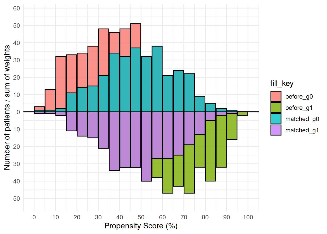
For a weighted analysis, pass the weight column and the bars become weighted counts.
mh_wt <- hvtiPlotR::hv_mirror_hist(w_ate$data,
                                   score_col  = "prob_t",
                                   group_col  = "tavr",
                                   weight_col = "iptw")
#> mirror_histogram diagnostics: n=800  dropped=0  [see $tables$diagnostics]
plot(mh_wt)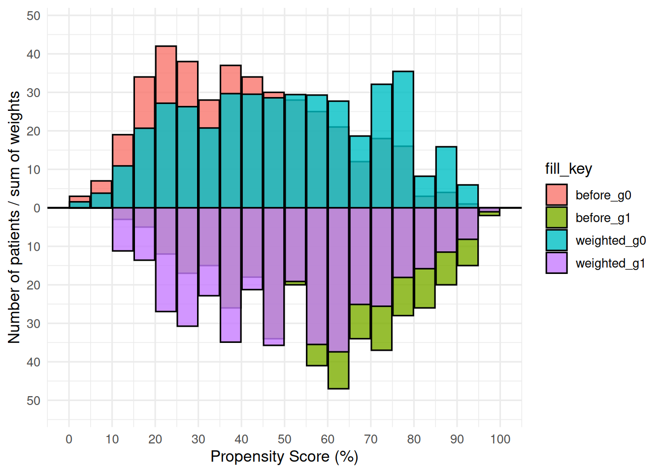
10.2 Covariate balance plot
hv_balance() does not read $tables as they come. It wants one long data frame, one row per covariate and comparison, with columns variable, group and std_diff, and the difference in percent (its reference lines sit at plus and minus 10). The SMD tables here are proportions of a standard deviation, one table per comparison, so stack them and multiply by 100. Here is the logit-scale match from earlier.
balance_long <- rbind(
  data.frame(variable = m_logit$tables$smd_before$variable,
             group    = "Before match",
             std_diff = 100 * m_logit$tables$smd_before$smd),
  data.frame(variable = m_logit$tables$smd_after$variable,
             group    = "After match",
             std_diff = 100 * m_logit$tables$smd_after$smd)
)
balance_long
#>        variable        group std_diff
#> 1           age Before match   -75.59
#> 2        female Before match    15.82
#> 3            ef Before match    55.09
#> 4      diabetes Before match   -12.57
#> 5  hypertension Before match    -6.96
#> 6           age  After match    -3.45
#> 7        female  After match    -7.50
#> 8            ef  After match    -2.07
#> 9      diabetes  After match    -3.43
#> 10 hypertension  After match     0.00
For a ps_weight() object the two tables are smd_unweighted and smd_weighted.
cb <- hvtiPlotR::hv_balance(balance_long)
plot(cb)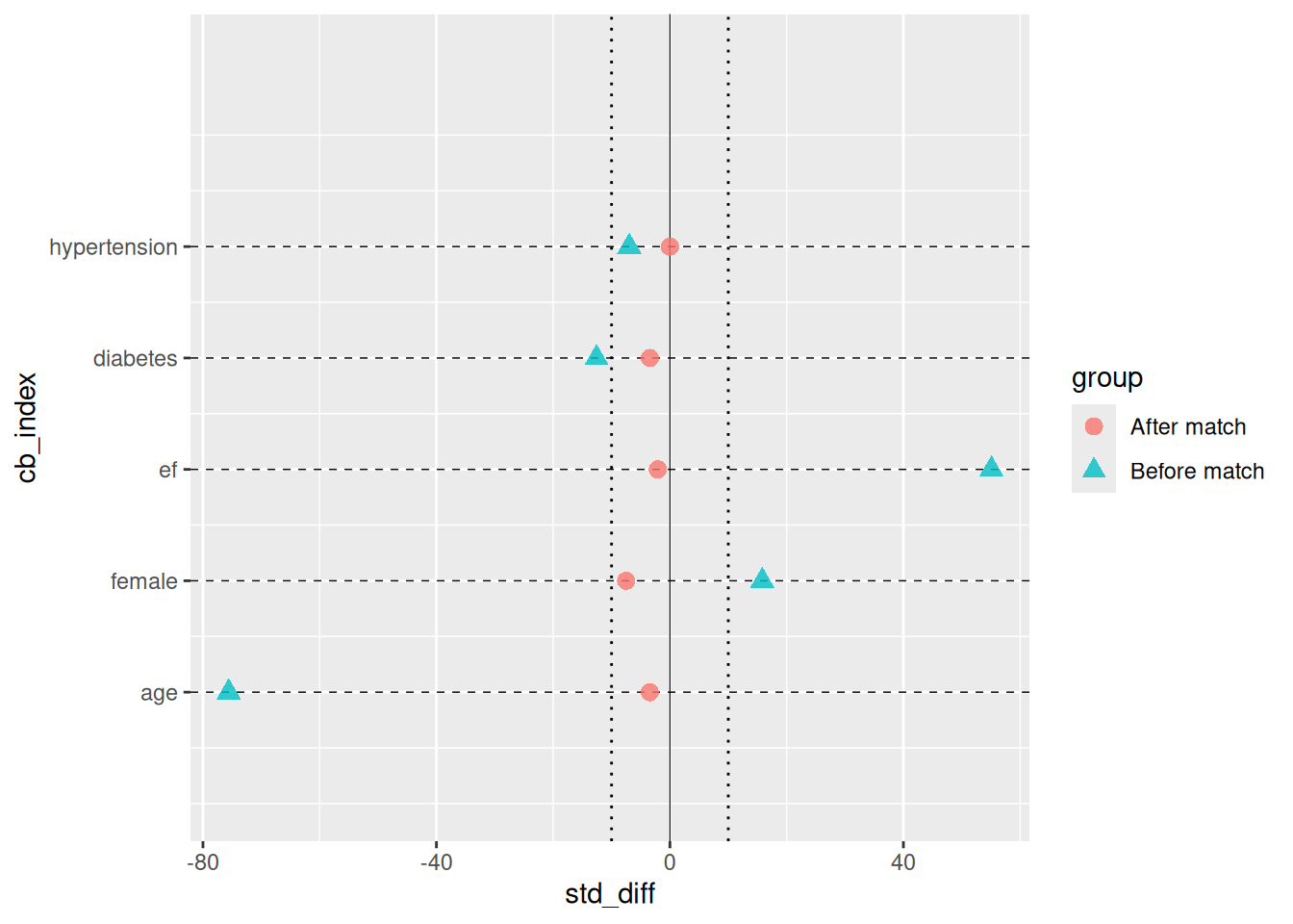
11 Session info
sessionInfo()
#> R version 4.6.1 (2026-06-24)
#> Platform: x86_64-pc-linux-gnu
#> Running under: Ubuntu 24.04.5 LTS
#>
#> Matrix products: default
#> BLAS:   /usr/lib/x86_64-linux-gnu/openblas-pthread/libblas.so.3
#> LAPACK: /usr/lib/x86_64-linux-gnu/openblas-pthread/libopenblasp-r0.3.26.so;  LAPACK version 3.12.0
#>
#> locale:
#>  [1] LC_CTYPE=C.UTF-8       LC_NUMERIC=C           LC_TIME=C.UTF-8
#>  [4] LC_COLLATE=C.UTF-8     LC_MONETARY=C.UTF-8    LC_MESSAGES=C.UTF-8
#>  [7] LC_PAPER=C.UTF-8       LC_NAME=C              LC_ADDRESS=C
#> [10] LC_TELEPHONE=C         LC_MEASUREMENT=C.UTF-8 LC_IDENTIFICATION=C
#>
#> time zone: UTC
#> tzcode source: system (glibc)
#>
#> attached base packages:
#> [1] stats     graphics  grDevices utils     datasets  methods   base
#>
#> other attached packages:
#> [1] hvtiRpropensity_0.2.1
#>
#> loaded via a namespace (and not attached):
#>  [1] gtable_0.3.6            xfun_0.61               ggplot2_4.0.3
#>  [4] hvtiPlotR_2.8.10        htmlwidgets_1.6.4       visNetwork_2.1.4
#>  [7] lattice_0.22-9          vctrs_0.7.3             tools_4.6.1
#> [10] generics_0.1.4          parallel_4.6.1          tibble_3.3.1
#> [13] pkgconfig_2.0.3         Matrix_1.7-5            RColorBrewer_1.1-3
#> [16] S7_0.2.2                rvg_0.4.2               randomForestSRC_3.9.0
#> [19] uuid_1.2-2              ggupset_0.4.1           lifecycle_1.0.5
#> [22] compiler_4.6.1          farver_2.1.2            textshaping_1.0.5
#> [25] data.tree_1.2.0         fontquiver_0.2.1        fontLiberation_0.1.0
#> [28] htmltools_0.5.9         yaml_2.3.12             pillar_1.11.1
#> [31] tidyr_1.3.2             MASS_7.3-65             openssl_2.4.2
#> [34] fontBitstreamVera_0.1.1 tidyselect_1.2.1        zip_3.0.2
#> [37] digest_0.6.39           stringi_1.8.9           dplyr_1.2.1
#> [40] purrr_1.2.2             labeling_0.4.3          splines_4.6.1
#> [43] fastmap_1.2.0           grid_4.6.1              cli_3.6.6
#> [46] magrittr_2.0.5          DiagrammeR_1.0.12       patchwork_1.3.2
#> [49] survival_3.8-6          withr_3.0.3             gdtools_0.5.1
#> [52] scales_1.4.0            consort_1.2.4           rmarkdown_2.32
#> [55] officer_0.7.6           otel_0.2.0              nnet_7.3-20
#> [58] askpass_1.2.1           ragg_1.5.2              ggalluvial_0.12.6
#> [61] evaluate_1.0.5          knitr_1.52              rlang_1.3.0
#> [64] Rcpp_1.1.2              glue_1.8.1              xml2_1.6.0
#> [67] jsonlite_2.0.0          R6_2.6.1                systemfonts_1.3.2