Late-phase (G3) temporal decomposition

Computes the cumulative intensity $G_3(t)$ and its derivative $g_3(t) = dG_3/dt$ for the late-phase parametric family used in the original Blackstone C/SAS HAZARD code. Unlike hzr_decompos() (which computes the early-phase G1 – a bounded CDF), this function can produce unbounded values, making it suitable for modelling increasing late risk.

Usage

hzr_decompos_g3(time, tau, gamma, alpha, eta)

Arguments

time: Numeric vector of times (must be > 0).
tau: Positive scalar scale parameter.
gamma: Positive scalar time exponent.
alpha: Non-negative scalar shape parameter (0 selects limiting case).
eta: Positive scalar outer exponent.

Value

A named list with two numeric vectors, each the same length as time:

G3: Cumulative intensity $G_3(t) \ge 0$ (may exceed 1).
g3: Derivative $g_3(t) = dG_3/dt \ge 0$.

Mathematical form

When $\alpha > 0$: $$G_3(t) = \bigl(\bigl((t/\tau)^\gamma + 1\bigr)^{1/\alpha} - 1\bigr)^\eta$$

When $\alpha = 0$ (limiting exponential case): $$G_3(t) = \bigl(\exp\bigl((t/\tau)^\gamma\bigr) - 1\bigr)^\eta$$

Parameter mapping from SAS/C HAZARD

SAS name	R argument	Role
TAU	`tau`	Scale (time at which $(t/\tau) = 1$)
GAMMA	`gamma`	Power exponent on $t/\tau$
ALPHA	`alpha`	Shape (0 = exponential limiting case)
ETA	`eta`	Outer power exponent

References

Blackstone EH, Naftel DC, Turner ME Jr. The decomposition of time-varying hazard into phases, each incorporating a separate stream of concomitant information. J Am Stat Assoc. 1986;81(395):615–624. doi:10.1080/01621459.1986.10478314

Examples

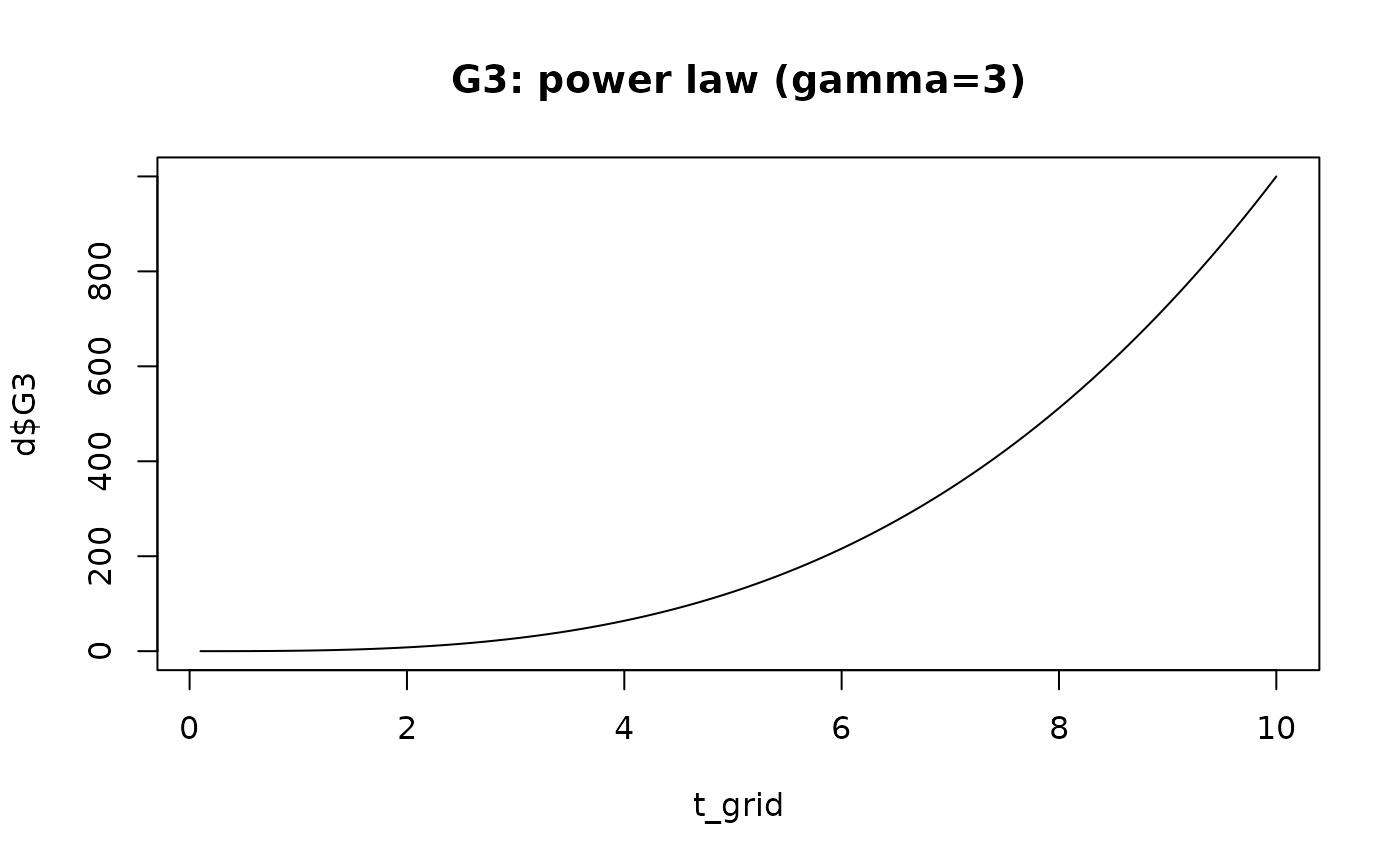
t_grid <- seq(0.1, 10, by = 0.1)

# Weibull-like: alpha = 1 gives G3(t) = (t/tau)^(gamma*eta)
d <- hzr_decompos_g3(t_grid, tau = 1, gamma = 3, alpha = 1, eta = 1)
plot(t_grid, d$G3, type = "l", main = "G3: power law (gamma=3)")


# General case with alpha > 0
d2 <- hzr_decompos_g3(t_grid, tau = 2, gamma = 2, alpha = 0.5, eta = 1)