Fitting Hazard Models
From intercept-only to multiphase additive hazard
Source:vignettes/fitting-hazard-models.qmd
This vignette walks the core model-fitting workflow from the inside out: intercept-only fits to establish the baseline hazard shape, then covariates on top, then the multiphase decomposition, then multi-endpoint analyses on the same cohort. Every example uses a clinical dataset shipped with the package. If you haven’t seen the basics — what a parametric hazard model is, why we use the Surv(time, status) formula — start with vignette("getting-started") first; this vignette assumes that context.
The progression matters. Single-distribution intercept-only fits tell you whether the baseline hazard shape is monotone (Weibull territory) or has structure that demands a multiphase decomposition. Multivariable fits add covariate effects on top of a shape you already trust. Multiphase fits split the baseline shape into clinically interpretable phases. Multi-endpoint analyses reuse all the above for separate clinical outcomes — death, reoperation, infection — on the same patient cohort.
1 Intercept-only model: CABG survival (KU Leuven)
The cabgkul dataset contains 5,880 patients who underwent primary isolated coronary artery bypass grafting at KU Leuven between 1971 and 1987. With only two columns — follow-up time and death indicator — it is the simplest starting point.
Fit an intercept-only Weibull. With no covariates on the right-hand side of the formula the model estimates only the baseline hazard shape — the scale mu and exponent nu of a Weibull curve fit to all 5,880 patients pooled. This is the right starting point for any new dataset: before asking which covariates matter, ask whether a single monotone hazard even fits the population-level pattern.
The summary tells us where the optimizer landed; the picture tells us whether that landing point matches the data. Plot the fitted survival curve on a fine time grid and overlay the Kaplan-Meier step function from the raw cohort.
t_grid <- seq(0.01, max(cabgkul$int_dead) * 0.9, length.out = 200)
nd     <- data.frame(time = t_grid)
surv   <- predict(fit_kul, newdata = nd, type = "survival") * 100

km     <- survfit(Surv(int_dead, dead) ~ 1, data = cabgkul)
km_df  <- data.frame(time = km$time, survival = km$surv * 100)

ggplot() +
  geom_step(data = km_df, aes(time, survival, colour = "Kaplan-Meier"),
            linewidth = 0.5) +
  geom_line(data = data.frame(time = t_grid, survival = surv),
            aes(time, survival, colour = "Weibull"), linewidth = 1) +
  scale_colour_manual(values = c("Weibull" = "#0072B2",
                                 "Kaplan-Meier" = "#D55E00")) +
  scale_y_continuous(limits = c(0, 100)) +
  labs(x = "Months after CABG", y = "Freedom from death (%)",
       colour = NULL) +
  theme_minimal() +
  theme(legend.position = "bottom")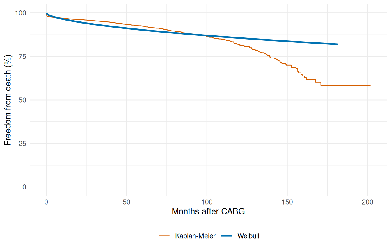
A single Weibull captures the broad trend but misses the distinct early operative risk and late attrition that the KM curve reveals. This motivates the multiphase approach below.
2 Multivariable model: AVC repair
The avc dataset has 310 patients who underwent atrioventricular canal repair, with 9 candidate covariates spanning patient demographics (age, NYHA status), anatomical features (malalignment, orifice morphology), intra-operative grading (inc_surg = surgical grade of AV valve incompetence), and post-operative complications (com_iv = grade IV complications). We drop incomplete rows so the design matrix is rectangular, then look at the column types and ranges.
data(avc)
avc <- na.omit(avc)
str(avc)
#> 'data.frame':    305 obs. of  11 variables:
#>  $ study   : chr  "001C" "002C" "004C" "005C" ...
#>  $ status  : int  3 3 1 2 2 3 1 1 3 3 ...
#>  $ inc_surg: int  4 3 2 3 1 2 3 2 3 3 ...
#>  $ opmos   : num  9.46 34.07 51.58 55 60.65 ...
#>  $ age     : num  69.2 53.7 286.1 154.6 48.4 ...
#>  $ mal     : int  0 0 0 1 0 0 0 0 0 0 ...
#>  $ com_iv  : int  1 1 1 1 1 1 1 1 1 1 ...
#>  $ orifice : int  0 0 0 0 0 0 0 0 0 0 ...
#>  $ dead    : int  1 1 0 0 0 0 0 0 0 1 ...
#>  $ int_dead: num  0.0534 0.3778 91.5337 111.608 106.8112 ...
#>  $ op_age  : num  654 1828 14759 8505 2933 ...
#>  - attr(*, "na.action")= 'omit' Named int [1:5] 12 90 138 144 146
#>   ..- attr(*, "names")= chr [1:5] "12" "90" "138" "144" ...
Now we put covariates on the right-hand side of the formula and refit. The theta vector grows: two Weibull shape parameters (mu, nu) plus six covariate coefficients (beta1..beta6), each starting at zero. The optimizer estimates a log-hazard-ratio for every covariate jointly with the Weibull shape — so the shape and the covariate effects are identified from the same likelihood, not sequentially.
fit_avc <- hazard(
  Surv(int_dead, dead) ~ age + status + mal + com_iv + inc_surg + orifice,
  data  = avc,
  dist  = "weibull",
  theta = c(mu = 0.20, nu = 1.0, rep(0, 6)),
  fit   = TRUE,
  control = list(maxit = 500)
)

fit_avc
#> hazard object
#>   observations: 305
#>   predictors:   6
#>   dist:         weibull
#>   engine:       native-r-m2
#>   log-lik:      -197.159
#>   converged:    TRUE
Each coefficient is a log-hazard-ratio: positive means higher risk, negative means lower, zero means no effect. The large positive coefficients on mal (anatomical malalignment) and com_iv (grade IV post-operative complications) flag these as the dominant risk markers in this cohort. The standard errors and Wald z-statistics in the summary tell you which effects are well identified and which are noise — a coefficient with a z-statistic near zero contributes essentially nothing the data can defend.
3 Multiphase model: additive hazard decomposition
The single-Weibull fits above gave us a curve that’s mediocre everywhere instead of right anywhere. That’s a structural limitation of a monotone parametric shape, not something more iterations will fix. The Blackstone–Naftel–Turner framework’s key idea is to split the hazard into a sum of phase-specific contributions, each with its own temporal shape and its own scale:
\[H(t \mid x) = \sum_{j=1}^{J} \mu_j(x) \cdot \Phi_j(t)\]
Each \(\Phi_j(t)\) is a phase-specific unit-scaled curve (early-peaking saturating, flat constant, late-rising polynomial) and each \(\mu_j(x)\) is the phase-specific scale, possibly modulated by covariates. The phases overlap and add — no switching, no thresholds — so the total instantaneous hazard at any \(t\) is the sum of the per-phase rates. See vignette("getting-started") for the longer-form motivation; what follows here is the practical workflow for fitting one.
For AVC we’ll use two phases — an early phase to absorb the operative-window mortality, and a constant phase for the background rate. AVC patients don’t have a clear late-deterioration regime over this follow-up window, so a third (g3) phase would be unidentified. We fix the shape parameters and estimate only the scales, matching the workflow you’d run against a SAS HAZARD reference fit.
fit_mp <- hazard(
  Surv(int_dead, dead) ~ 1,
  data   = avc,
  dist   = "multiphase",
  phases = list(
    early    = hzr_phase("cdf", t_half = 0.5, nu = 1, m = 1,
                          fixed = "shapes"),
    constant = hzr_phase("constant")
  ),
  fit     = TRUE,
  control = list(n_starts = 5, maxit = 1000)
)
#> Warning in .hzr_optim_generic(logl_fn = logl_fn, gradient_fn = gradient_fn, :
#> hessian_fn returned a non-conformant result; using numerical Hessian
#> Warning in .hzr_optim_generic(logl_fn = logl_fn, gradient_fn = gradient_fn, :
#> hessian_fn returned a non-conformant result; using numerical Hessian
#> Warning in .hzr_optim_generic(logl_fn = logl_fn, gradient_fn = gradient_fn, :
#> hessian_fn returned a non-conformant result; using numerical Hessian
#> Warning in .hzr_optim_generic(logl_fn = logl_fn, gradient_fn = gradient_fn, :
#> hessian_fn returned a non-conformant result; using numerical Hessian
#> Warning in .hzr_optim_generic(logl_fn = logl_fn, gradient_fn = gradient_fn, :
#> hessian_fn returned a non-conformant result; using numerical Hessian

summary(fit_mp)
#> Multiphase hazard model (2 phases)
#>   observations: 305
#>   predictors:   0
#>   dist:         multiphase
#>   phase 1:      early - cdf (early risk)
#>   phase 2:      constant - constant (flat rate)
#>   engine:       native-r-m2
#>   converged:    TRUE
#>   log-lik:      -228.029
#>   evaluations: fn=32, gr=10
#>
#> Coefficients (internal scale):
#>
#>   Phase: early (cdf)
#>                estimate std_error    z_stat     p_value
#>   log_mu     -1.4132735 0.1290435 -10.95192 6.50568e-28
#>   log_t_half -0.6931472        NA        NA          NA
#>   nu          1.0000000        NA        NA          NA
#>   m           1.0000000        NA        NA          NA
#>
#>   Phase: constant (constant)
#>           estimate std_error    z_stat      p_value
#>   log_mu -7.609476 0.4495827 -16.92564 2.911483e-64
The diagnostic that matters is whether the multiphase fit actually out-performs the single Weibull against the data. Plot both parametric curves against the same Kaplan-Meier reference so we can see, by eye, where each model is honest and where each is reaching.
t_grid <- seq(0.01, max(avc$int_dead) * 0.95, length.out = 200)
nd     <- data.frame(time = t_grid)

km_avc <- survfit(Surv(int_dead, dead) ~ 1, data = avc)
km_df  <- data.frame(time = km_avc$time, survival = km_avc$surv * 100)

fit_wb <- hazard(
  Surv(int_dead, dead) ~ 1, data = avc, dist = "weibull",
  theta = c(mu = 0.20, nu = 1.0), fit = TRUE
)

surv_wb <- predict(fit_wb, newdata = nd, type = "survival") * 100
surv_mp <- predict(fit_mp, newdata = nd, type = "survival") * 100

plot_df <- rbind(
  data.frame(time = t_grid, survival = surv_wb, Model = "Single Weibull"),
  data.frame(time = t_grid, survival = surv_mp, Model = "Multiphase (2-phase)")
)

ggplot() +
  geom_step(data = km_df, aes(time, survival), colour = "grey50",
            linewidth = 0.5) +
  geom_line(data = plot_df, aes(time, survival, colour = Model),
            linewidth = 1) +
  scale_colour_manual(values = c("Single Weibull" = "#E69F00",
                                 "Multiphase (2-phase)" = "#0072B2")) +
  scale_y_continuous(limits = c(0, 100)) +
  annotate("text", x = max(t_grid) * 0.6, y = 95, label = "KM (grey)",
           size = 3, colour = "grey50") +
  labs(x = "Months after AVC repair", y = "Freedom from death (%)",
       colour = NULL) +
  theme_minimal() +
  theme(legend.position = "bottom")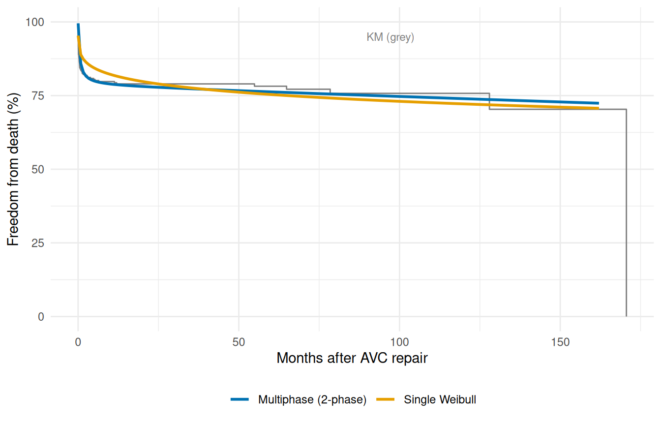
The multiphase model tracks the KM curve much more closely than the single Weibull, especially across the steep early-mortality window — which is exactly where the single Weibull was forced to compromise. The constant phase then carries the slow post-recovery attrition. The point isn’t that multiphase always wins; it’s that when the data has phase structure, fitting that structure explicitly is strictly more honest than averaging it away into one monotone curve.
4 Multi-endpoint models: heart valve replacement
The valves dataset (1,533 patients) has multiple time-to-event endpoints — death, prosthetic valve endocarditis (PVE), and reoperation — each with its own follow-up time and event indicator. The same hazard() call fits each endpoint independently:
Start with the death endpoint. We use age at operation, NYHA class, and mechanical-valve indicator as covariates — the clinically canonical set for survival after valve replacement.
data(valves)
valves <- na.omit(valves)

fit_death <- hazard(
  Surv(int_dead, dead) ~ age_cop + nyha + mechvalv,
  data  = valves,
  dist  = "weibull",
  theta = c(mu = 0.10, nu = 1.0, rep(0, 3)),
  fit   = TRUE,
  control = list(maxit = 500)
)

fit_death
#> hazard object
#>   observations: 1523
#>   predictors:   3
#>   dist:         weibull
#>   engine:       native-r-m2
#>   log-lik:      -1820.55
#>   converged:    TRUE
Switch endpoints. Same data, same package, but now we model time to prosthetic valve endocarditis instead of death. The covariate list shifts to match the clinical question: nve (native-valve endocarditis history) replaces nyha because functional class is less informative for infection risk than prior endocarditis exposure. The fit returns its own MLE, coefficients, and standard errors completely independent of the death model.
fit_pve <- hazard(
  Surv(int_pve, pve) ~ age_cop + nve + mechvalv,
  data  = valves,
  dist  = "weibull",
  theta = c(mu = 0.02, nu = 1.0, rep(0, 3)),
  fit   = TRUE,
  control = list(maxit = 500)
)

fit_pve
#> hazard object
#>   observations: 1523
#>   predictors:   3
#>   dist:         weibull
#>   engine:       native-r-m2
#>   log-lik:      -391.125
#>   converged:    TRUE
Each endpoint gets its own model with its own covariates, but the hazard model structure — temporal shape plus covariate effects — stays the same whatever the clinical endpoint. Repeating the workflow for a third endpoint (reoperation, for example) is mechanical: swap the Surv(...) columns, swap the covariates, refit. The advantage over running three separate analyses in different tools is that the predictions, diagnostics, and uncertainty quantification all come from the same package — there’s no risk of subtle differences in censoring handling or estimator choice between endpoints.
5 Interval and left censoring
Right censoring is by far the most common censoring type in clinical survival data — a patient is still alive at last follow-up, so all we know is that their event time exceeds the observed window. Two other types arise frequently enough to warrant explicit handling.
Interval censoring occurs when the event is known to have happened between two observation times, but not at a specific time. The canonical example is clinic-visit data: a patient is confirmed alive at month 12 and found dead at month 24, so the event occurred somewhere in \((12, 24)\). A naive analysis treats the event as right-censored at 12 or exactly observed at 24; both introduce bias.
Left censoring is the mirror: the event occurred before the first observation time (time_upper), so it was already established at the moment of first contact — \(T \leq t_{\text{upper}}\).
5.1 Status codes
The package encodes censoring type in the status vector:
| Status | Type | Interpretation |
|---|---|---|
1 |
Exact event | Observed at time
|
0 |
Right-censored | Event did not occur by time
|
2 |
Interval-censored | Event occurred in (time_lower, time_upper)
|
-1 |
Left-censored | Event occurred before time (upper bound) |
For interval-censored rows, supply both time_lower and time_upper directly to hazard(). The formula interface handles Surv(time, status) for right-censored data and Surv(start, stop, event) for counting-process (repeating-event) data; interval censoring is passed via the direct arguments.
5.2 Mixed censoring example
We simulate 400 cardiac surgery patients observed at semi-annual clinic visits (every 6 months, 4–8 scheduled visits per patient). If the event falls between two consecutive visits the observation is interval-censored; if it falls after the last visit the patient is right-censored.
set.seed(101)
n         <- 400
visit_gap <- 6   # months between visits

# True event times: Weibull mu = 0.025, nu = 1.0 (median ~28 months)
true_time <- rexp(n, rate = 0.025)  # nu=1 → exponential

n_visits  <- sample(4:8, n, replace = TRUE)

status     <- integer(n)
time       <- numeric(n)
time_lower <- numeric(n)
time_upper <- numeric(n)

for (i in seq_len(n)) {
  visits <- seq(visit_gap, n_visits[i] * visit_gap, by = visit_gap)
  t_ev   <- true_time[i]
  brk    <- findInterval(t_ev, c(0, visits))  # which interval contains t_ev

  if (brk > length(visits)) {
    # Event after last visit: right-censored.
    # time_lower = 0: with H(time_lower) = H(0) = 0, the right-censored
    # contribution reduces to -(H(time) - H(0)) = -H(time), which is correct.
    status[i]     <- 0L
    time[i]       <- max(visits)
    time_lower[i] <- 0
    time_upper[i] <- max(visits)
  } else {
    # Event within the visit window: interval-censored in (lower, upper)
    lower_bound   <- if (brk == 1L) 0 else visits[brk - 1L]
    upper_bound   <- visits[brk]
    status[i]     <- 2L
    time[i]       <- lower_bound
    time_lower[i] <- lower_bound
    time_upper[i] <- upper_bound
  }
}

table(status)
#> status
#>   0   2
#> 168 232
Note
time_loweras a counting-process entry time. In the Weibull and multiphase likelihoods,time_lowerdoubles as the entry (left-truncation) time for right-censored and exact-event rows (status %in% c(0, 1)): when0 < time_lower < time, the row contributes H(stop) − H(start), the counting-process form used for epoch-decomposed repeated events. For an ordinary right-censored or event row with no entry time, leavetime_lowerat0or omit it. Settingtime_lower = timeis treated as no entry —time_loweracts as an entry time only when strictly less thantime, so it no longer zeroes the row’s contribution. The exponential, log-logistic, and log-normal likelihoods do not usetime_loweras an entry time and are unaffected.
Fit a Weibull model using both censoring types:
fit_ic <- hazard(
  time       = time,
  status     = status,
  time_lower = time_lower,
  time_upper = time_upper,
  dist  = "weibull",
  theta = c(mu = 0.025, nu = 1.0),
  fit   = TRUE
)

fit_ic
#> hazard object
#>   observations: 400
#>   predictors:   0
#>   dist:         weibull
#>   engine:       native-r-m2
#>   log-lik:      -674.374
#>   converged:    TRUE
5.3 Interval-censored vs naive right-censored
A naive analyst who doesn’t have visit-bracket data would record the death at the discovery visit (time_upper) rather than as an interval. This overstates the event time — the patient appears to have survived longer than they did — biasing the estimated hazard shape.
# Naive: treat each interval-censored row as an exact event at time_upper
# (the visit when the death was first recorded)
fit_naive <- hazard(
  time   = ifelse(status == 2L, time_upper, time),
  status = ifelse(status == 2L, 1L,         status),
  dist  = "weibull",
  theta = c(mu = 0.025, nu = 1.0),
  fit   = TRUE
)

# Compare MLEs; true parameters are mu = 0.025, nu = 1.0
rbind(
  interval_censored = round(coef(fit_ic)[1:2],   4),
  naive_exact_upper = round(coef(fit_naive)[1:2], 4),
  truth             = c(mu = 0.025, nu = 1.0)
)
#>                       mu     nu
#> interval_censored 0.0251 1.0345
#> naive_exact_upper 0.0259 1.4566
#> truth             0.0250 1.0000
The interval-censored fit recovers both parameters accurately. The naive fit estimates \(\mu\) comparably but introduces a substantial positive bias in \(\nu\) — it sees events consistently appearing at visit times (every 6 months) and infers a sharper, more periodic hazard shape that doesn’t match the underlying exponential structure.
6 Convergence troubleshooting
Multiphase models have more parameters than single-distribution fits, and the likelihood surface can be flat or multimodal when the data doesn’t strongly identify all of them. Most convergence problems trace back to one of three causes: poor starting values, too many free parameters for the data at hand, or a model that asks for a phase the data doesn’t contain. This section shows how to diagnose each and what to do about it.
6.1 Reading the KM cumulative hazard for starting values
For a Weibull model, the relationship between the starting values and the data is direct: because \(H(t) = (\mu t)^\nu\), taking logs gives \(\log H(t) = \nu \log t + \nu \log \mu\). Plot \(\log H(t)\) (the Nelson-Aalen cumulative hazard on the log scale) against \(\log t\) and fit a straight line; the slope is \(\hat\nu\) and the intercept is \(\hat\nu \log \hat\mu\).
nel <- hzr_nelson(cabgkul$int_dead, cabgkul$dead)

# Drop the zero-time boundary point before log-transforming
nel_clean <- nel[nel$time > 0 & nel$cumhaz > 0, ]
log_t <- log(nel_clean$time)
log_H <- log(nel_clean$cumhaz)

lm_fit  <- lm(log_H ~ log_t)
nu_hat  <- unname(coef(lm_fit)[2])
mu_hat  <- exp(unname(coef(lm_fit)[1]) / nu_hat)
c(mu = round(mu_hat, 4), nu = round(nu_hat, 4))
#>     mu     nu
#> 0.0001 0.4793
Those values are the Weibull starting point the data itself suggests. They won’t be the MLEs — the log-log line uses every event time equally, whereas the MLE weights by the likelihood — but they land the optimizer in a sensible neighbourhood and prevent false-convergence to a degenerate solution.
For multiphase models the reading is qualitative. Plot the KM cumulative hazard on the natural scale and look for kinks: a steep-then-flattening shape in the first few months signals an early phase whose t_half should sit in that early window; a steady linear rise afterwards signals a constant phase; a late upward curve beyond the flat region signals a late phase. Set t_half to roughly the time at which the early kink levels off, and set the constant phase scale mu to approximate the slope of the linear mid-section.
ggplot(data.frame(time = nel$time, cumhaz = nel$cumhaz),
       aes(time, cumhaz)) +
  geom_step(colour = "#D55E00", linewidth = 0.7) +
  labs(x = "Months after CABG", y = "Cumulative hazard") +
  theme_minimal()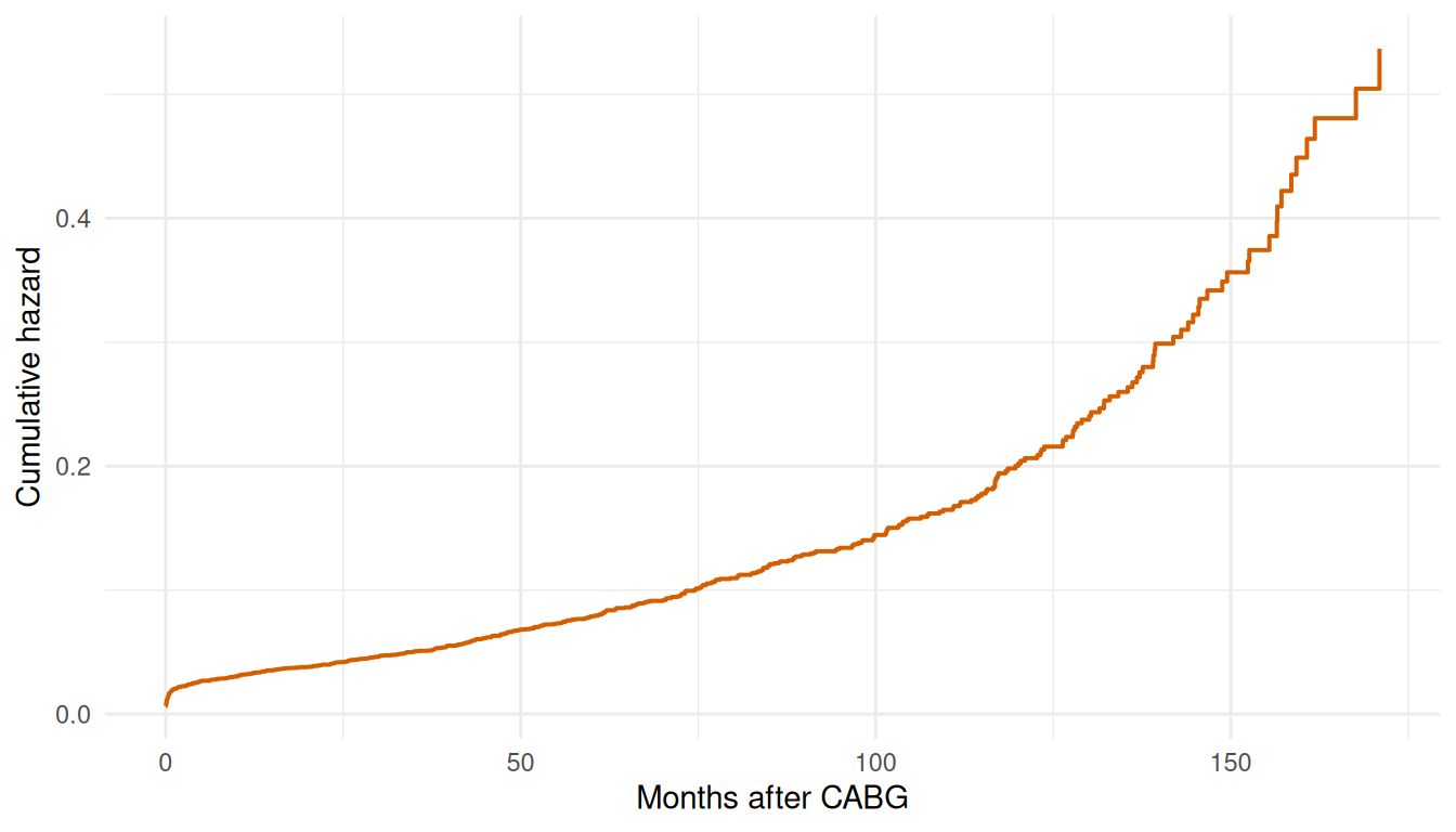
The early steep rise, the mid-range roughly-linear section, and the late upward acceleration map directly onto the three phases in the CABGKUL model.
6.2 When to fix shape parameters
fixed = "shapes" locks the temporal shape parameters (e.g., t_half, nu, m for a CDF phase; tau, gamma, alpha, eta for a g3 phase) and lets the optimizer estimate only the scale (log_mu) for each phase. This cuts the parameter count substantially and is almost always what you want in two situations:
- You have a reference fit. If a SAS HAZARD run already produced shape estimates, replicate those shapes exactly and re-estimate only the scale. This is the standard parity workflow.
- Your sample is small relative to the number of phases. A rough guide is 50 or more events per free shape parameter. Below that threshold the shapes are weakly identified and the optimizer wanders.
Estimate shapes freely (fixed = "none", the default) only when you are exploring a new dataset for the first time and have no prior on the temporal structure — and even then, start with fixed = "shapes" and release the shapes one at a time if the fixed-shapes fit shows systematic misfit.
6.3 Signs of overparameterization
When a model has more phases than the data supports, the symptoms are recognizable:
| Symptom | What it means |
|---|---|
fit$fit$converged == FALSE |
Optimizer hit maxit without satisfying the gradient tolerance |
vcov() returns NA
|
Hessian is singular — parameters are not jointly identified |
A phase scale (log_mu) at a boundary value |
That phase is contributing essentially zero hazard; it isn’t needed |
| Enormous standard errors on one or more parameters | Flat likelihood in that direction — weak identification |
| Two phases with nearly identical shapes | One can be collapsed into the other |
The AVC dataset has a clear two-phase structure (early CDF plus constant). Adding a third late-rising phase asks the data for a pattern it doesn’t contain over this follow-up window:
set.seed(42)
fit_3ph <- hazard(
  Surv(int_dead, dead) ~ 1,
  data   = avc,
  dist   = "multiphase",
  phases = list(
    early    = hzr_phase("cdf", t_half = 0.5, nu = 1, m = 1,
                          fixed = "shapes"),
    constant = hzr_phase("constant"),
    late     = hzr_phase("g3", tau = 5, gamma = 3, alpha = 1, eta = 1,
                          fixed = "shapes")
  ),
  fit = TRUE, control = list(n_starts = 5, maxit = 1000)
)
#> Warning in .hzr_safe_solve(H_unc): Hessian is ill-conditioned (rcond =
#> 4.46e-11); standard errors may be unreliable

# Scale magnitudes: exp(log_mu) ≈ 0 for any phase the data doesn't support
log_mu_idx <- grep("log_mu", names(coef(fit_3ph)))
round(exp(coef(fit_3ph)[log_mu_idx]), 6)
#>    early.log_mu constant.log_mu     late.log_mu
#>        0.248869        0.000000        0.000006
The constant and late phase scales are both near zero — the optimizer found no evidence in the AVC data for either of those temporal shapes over this follow-up window. The early phase is absorbing all the identifiable structure. Any phase whose fitted scale is \(\mu \lesssim 10^{-4}\) is not contributing meaningful hazard and is a candidate for removal. The right diagnostic question is not “did the AIC improve?” but “does this phase represent real clinical biology?” — late deterioration after AVC repair requires long follow-up to observe; this dataset doesn’t have it.
When shapes are also free (fixed = "none"), a redundant phase can make the Hessian rank-deficient and vcov() will return NA (the Hessian inversion failed). Fix by adding fixed = "shapes" to each phase to reduce the free-parameter count, then release shapes one at a time if the fixed-shapes fit shows systematic misfit.
6.4 Optimizer options
Three control arguments address most remaining convergence problems:
n_starts (default 5 for multiphase; single-distribution models run one optimizer call and ignore this parameter) runs the optimizer from n_starts randomly jittered copies of the initial theta, then keeps the best solution. The default of 5 is sufficient for two-phase models; increase to 8–10 for three or more phases where the likelihood surface has more local minima.
set.seed(42)
fit_robust <- hazard(
  Surv(int_dead, dead) ~ 1,
  data   = avc,
  dist   = "multiphase",
  phases = list(
    early    = hzr_phase("cdf", t_half = 0.5, nu = 1, m = 1,
                          fixed = "shapes"),
    constant = hzr_phase("constant")
  ),
  fit     = TRUE,
  control = list(n_starts = 10, maxit = 1000)
)
#> Warning in .hzr_optim_generic(logl_fn = logl_fn, gradient_fn = gradient_fn, :
#> hessian_fn returned a non-conformant result; using numerical Hessian
#> Warning in .hzr_optim_generic(logl_fn = logl_fn, gradient_fn = gradient_fn, :
#> hessian_fn returned a non-conformant result; using numerical Hessian
#> Warning in .hzr_optim_generic(logl_fn = logl_fn, gradient_fn = gradient_fn, :
#> hessian_fn returned a non-conformant result; using numerical Hessian
#> Warning in .hzr_optim_generic(logl_fn = logl_fn, gradient_fn = gradient_fn, :
#> hessian_fn returned a non-conformant result; using numerical Hessian
#> Warning in .hzr_optim_generic(logl_fn = logl_fn, gradient_fn = gradient_fn, :
#> hessian_fn returned a non-conformant result; using numerical Hessian
#> Warning in .hzr_optim_generic(logl_fn = logl_fn, gradient_fn = gradient_fn, :
#> hessian_fn returned a non-conformant result; using numerical Hessian
#> Warning in .hzr_optim_generic(logl_fn = logl_fn, gradient_fn = gradient_fn, :
#> hessian_fn returned a non-conformant result; using numerical Hessian
#> Warning in .hzr_optim_generic(logl_fn = logl_fn, gradient_fn = gradient_fn, :
#> hessian_fn returned a non-conformant result; using numerical Hessian
#> Warning in .hzr_optim_generic(logl_fn = logl_fn, gradient_fn = gradient_fn, :
#> hessian_fn returned a non-conformant result; using numerical Hessian
#> Warning in .hzr_optim_generic(logl_fn = logl_fn, gradient_fn = gradient_fn, :
#> hessian_fn returned a non-conformant result; using numerical Hessian
fit_robust$fit$converged
#> [1] TRUE
Optimizer strategy (automatic). The package always uses BFGS as the primary optimizer. For fixed-shape multiphase models with 2–10 free parameters, a Nelder-Mead pass runs first on each start to find a good basin, then BFGS polishes the solution. This warm-up is transparent — it happens automatically when the conditions are met and there is no user-facing control to switch it on or off.
maxit (default 1000) sets the BFGS iteration cap. Hitting maxit without converging usually means either the starting values are far from the optimum (fix with better starts or n_starts) or the model is overparameterized (fix by fixing shapes or dropping a phase). Raising maxit beyond 2000 rarely helps if the optimizer is genuinely stuck.
7 Phase types reference
You’ve now seen each phase type in use: a "cdf" early phase for AVC operative mortality, a "constant" phase for AVC background rate, and the implicit single shape of every Weibull fit. The package supports three phase types in total, summarized here for quick reference:
| Type | Description | Typical use |
|---|---|---|
"cdf" |
Sigmoidal CDF shape (parameterized by t_half, nu, m) |
Early or late phases with transient risk |
"constant" |
Flat hazard (no temporal shape parameters) | Ongoing background risk |
"g3" |
Late-phase G3 parameterization (4 parameters: tau, gamma, alpha, eta) |
Late-rising risk matching C/SAS G3 output |
The "cdf" type covers the widest range of shapes: setting t_half small (e.g., 0.5) creates an early-peaking phase; setting it large (e.g., 10) creates a late-rising phase. The "constant" phase needs no shape parameters. The "g3" shape is the explicit late-rising parameterization that matches the SAS HAZARD “late” library; use it when you need parity against a C/SAS reference fit, or when the late rise has a clear lag-then-accelerate pattern that a delayed "cdf" doesn’t capture cleanly. See vignette("mf-mathematical-foundations") for the full mathematical treatment of each, including the parameter identifiability constraints.