Mathematical Foundations of TemporalHazard

Generalized decomposition, multiphase additive hazard, censoring, and time-varying covariates

library(TemporalHazard)

This vignette provides the mathematical foundation for the models implemented in TemporalHazard. It covers the generalized temporal decomposition family (Blackstone, Naftel, and Turner 1986), the additive multiphase hazard model, maximum likelihood estimation under mixed censoring, and extensions for time-varying covariates. The decomposition framework extends naturally to longitudinal mixed-effects settings (Rajeswaran et al. 2018).

For users migrating from the legacy SAS/C HAZARD program, each section notes how the R parameterization relates to the original parameter names. For the full translation table, see vignette("sas-to-r-migration") or call hzr_argument_mapping().

1 Generalized Temporal Decomposition

1.1 The parametric family

Every temporal phase in TemporalHazard is built from a single parametric family, decompos(t; t_half, nu, m), introduced by Blackstone, Naftel, and Turner (1986) that produces three linked quantities from just three parameters:

• $G(t)$ — cumulative distribution function (CDF), bounded $[0, 1]$
• $g(t) = dG/dt$ — probability density function
• $h(t) = g(t) / (1 - G(t))$ — hazard function

The three parameters control the shape of the distribution:

Parameter	Meaning	Constraint
t_half	Half-life: time at which $G(t_{1/2}) = 0.5$	$> 0$
nu	Time exponent — controls rate dynamics	any finite value
m	Shape exponent — controls distributional form	any finite value

SAS/C parameter bridge

The original C code used different parameter names per phase:

• Early phase (G1): DELTA, RHO/THALF, NU, M $\to$t_half, nu, m
• Late phase (G3): TAU, GAMMA, ALPHA, ETA $\to$t_half, nu, m

Both collapse onto the same 3-parameter decomposition family. The C DELTA parameter controlled a time transformation $B(t) = (\exp(\delta t) - 1)/\delta$ that is absorbed into the shape.

In R, hzr_decompos() computes all three quantities:

t_grid <- seq(0.01, 10, length.out = 200)

# Standard sigmoidal (Case 1: m > 0, nu > 0)
d <- hzr_decompos(t_grid, t_half = 3, nu = 2, m = 1)

# Verify the half-life property: G(t_half) = 0.5
d_half <- hzr_decompos(3, t_half = 3, nu = 2, m = 1)
cat("G(t_half) =", round(d_half$G, 6), "\n")
#> G(t_half) = 0.5

# Verify the identity: h(t) = g(t) / (1 - G(t))
h_check <- d$g / (1 - d$G)
cat("Max |h - g/(1-G)| =", max(abs(d$h - h_check)), "\n")
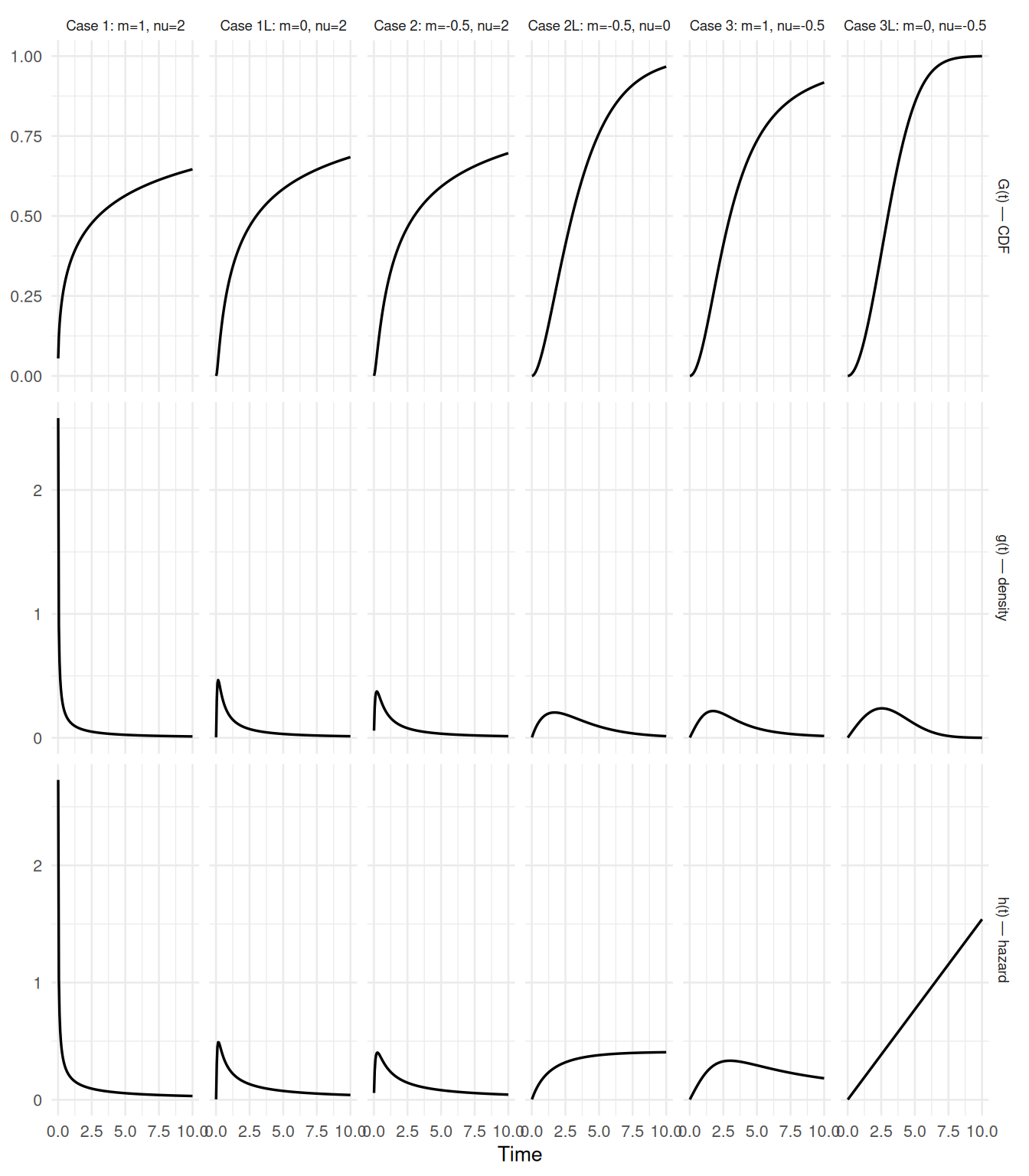
#> Max |h - g/(1-G)| = 0

1.2 The six valid cases

The signs of nu and m determine six distinct distributional shapes. The combination $m < 0$and $\nu < 0$ is undefined and raises an error.

Six valid parameter sign combinations

Case	m	nu	Behavior
1	> 0	> 0	Standard sigmoidal
1L	= 0	> 0	Weibull-like (exponential limit as m -> 0)
2	< 0	> 0	Heavy-tailed
2L	< 0	= 0	Exponential decay
3	> 0	< 0	Bounded cumulative
3L	= 0	< 0	Bounded exponential

The following plot shows the CDF $G(t)$, density $g(t)$, and hazard $h(t)$ for each case, all with t_half = 3:

if (has_ggplot) {
  library(ggplot2)

  params <- list(
    "Case 1: m=1, nu=2"     = list(nu = 2,   m = 1),
    "Case 1L: m=0, nu=2"    = list(nu = 2,   m = 0),
    "Case 2: m=-0.5, nu=2"  = list(nu = 2,   m = -0.5),
    "Case 2L: m=-0.5, nu=0" = list(nu = 0,   m = -0.5),
    "Case 3: m=1, nu=-0.5"  = list(nu = -0.5, m = 1),
    "Case 3L: m=0, nu=-0.5" = list(nu = -0.5, m = 0)
  )

  t_grid <- seq(0.01, 10, length.out = 200)
  rows <- list()

  for (nm in names(params)) {
    p <- params[[nm]]
    d <- hzr_decompos(t_grid, t_half = 3, nu = p$nu, m = p$m)
    rows <- c(rows, list(data.frame(
      time = rep(t_grid, 3),
      value = c(d$G, d$g, d$h),
      quantity = rep(c("G(t) — CDF", "g(t) — density", "h(t) — hazard"),
                     each = length(t_grid)),
      case = nm
    )))
  }

  df <- do.call(rbind, rows)

  # Cap hazard display at reasonable values for readability
  df$value[df$quantity == "h(t) — hazard" & df$value > 5] <- NA

  ggplot(df, aes(x = time, y = value)) +
    geom_line(linewidth = 0.6) +
    facet_grid(quantity ~ case, scales = "free_y") +
    labs(x = "Time", y = NULL) +
    theme_minimal(base_size = 10) +
    theme(strip.text = element_text(size = 7))
}

Figure 1: G(t), g(t), and h(t) for all six valid decomposition cases

1.3 Derivation sketch

The construction begins with a rate function $\rho$ chosen so that $G(t_{1/2}) = 0.5$ exactly. For Case 1 ($m > 0, \nu > 0$):

$$\rho = \nu \, t_{1/2} \left(\frac{2^m - 1}{m}\right)^{\!\nu}$$

Then, with the dimensionless time $b(t) = \nu t / \rho$:

$$G(t) = \left(1 + m \, b(t)^{-1/\nu}\right)^{-1/m}$$

$$g(t) = \left(1 + m \, b(t)^{-1/\nu}\right)^{-1/m - 1} \cdot b(t)^{-1/\nu - 1} / \rho$$

The other five cases arise as limits ($m \to 0$, $\nu \to 0$) or sign reflections of this base form. The implementation in hzr_decompos() dispatches to the appropriate branch after checking the signs of nu and m.

2 Additive Multiphase Hazard Model

2.1 Model specification

The total cumulative hazard decomposes additively across $J$ phases:

$$H(t \mid \mathbf{x}) = \sum_{j=1}^{J} \mu_j(\mathbf{x}) \cdot \Phi_j(t;\, t_{1/2,j},\, \nu_j,\, m_j)$$

where:

• $\mu_j(\mathbf{x}) = \exp(\alpha_j + \mathbf{x}_j \boldsymbol{\beta}_j)$ is the phase-specific log-linear scale with covariates
• $\Phi_j(t)$ is the temporal shape, determined by the phase type

The three phase types correspond to different uses of the decomposition output:

Phase type	$\Phi_j(t)$	Domain	Interpretation
"cdf"	$G(t)$	$[0, 1]$	Early risk that resolves over time
"hazard"	$-\log(1 - G(t))$	$[0, \infty)$	Late or aging risk that accumulates
"constant"	$t$	$[0, \infty)$	Flat background rate (no shape parameters)

SAS/C bridge

The classic three-phase HAZARD model used:

• G1 (early) $\to$hzr_phase("cdf", ...)
• G2 (constant) $\to$hzr_phase("constant")
• G3 (late) $\to$hzr_phase("hazard", ...)

TemporalHazard generalizes this to $N$ phases of any type.

2.2 Derived quantities

From the cumulative hazard, the instantaneous hazard and survival are:

$$h(t \mid \mathbf{x}) = \sum_{j=1}^{J} \mu_j(\mathbf{x}) \cdot \varphi_j(t) \qquad\text{where } \varphi_j = d\Phi_j/dt$$

$$S(t \mid \mathbf{x}) = \exp\!\bigl(-H(t \mid \mathbf{x})\bigr)$$

The derivative $\varphi_j(t)$ depends on phase type:

• "cdf": $\varphi(t) = g(t)$ (the density)
• "hazard": $\varphi(t) = h(t) = g(t)/(1 - G(t))$
• "constant": $\varphi(t) = 1$

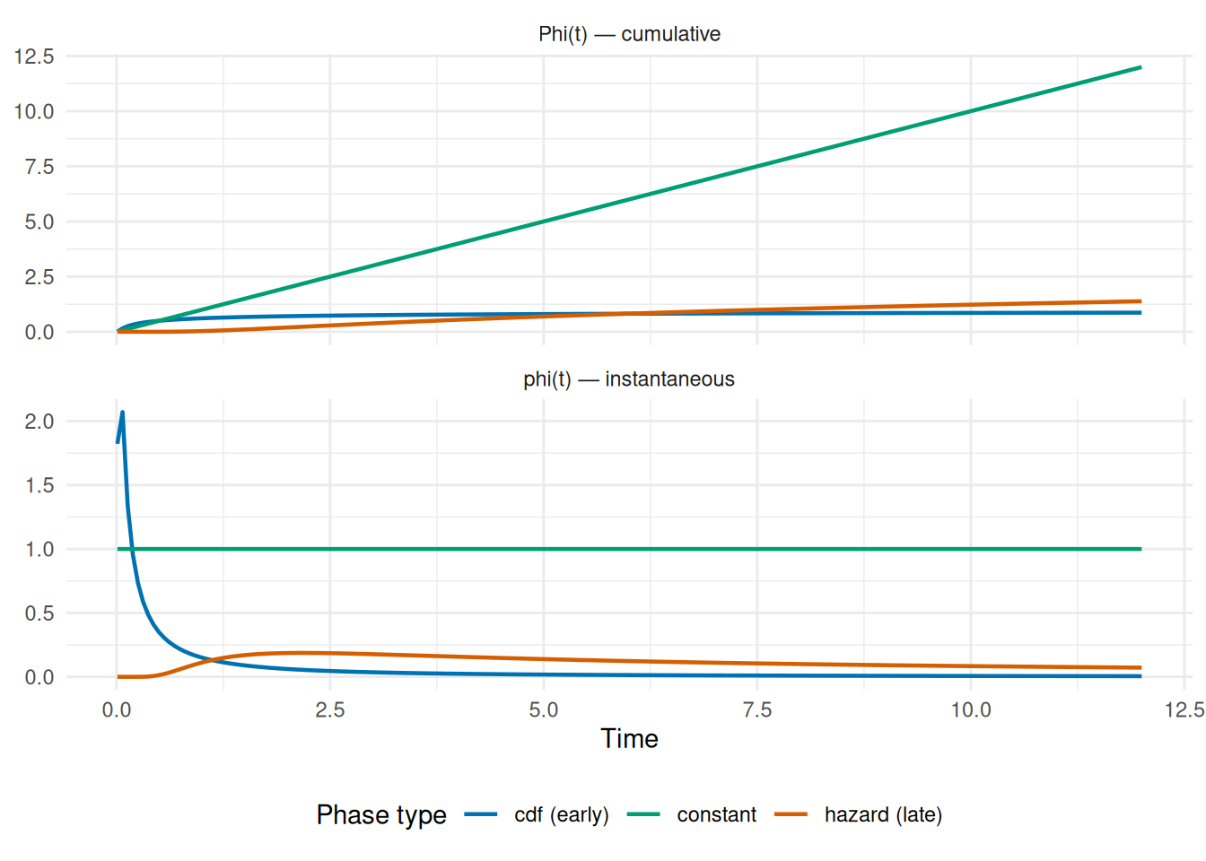
2.3 Constructing phases in R

Each phase is specified with hzr_phase() and passed to hazard():

# Classic three-phase pattern
early <- hzr_phase("cdf",      t_half = 0.5, nu = 2, m = 0)
const <- hzr_phase("constant")
late  <- hzr_phase("hazard",   t_half = 5,   nu = 1, m = 0)

print(early)
#> <hzr_phase> cdf (early risk) 
#>   t_half = 0.5  nu = 2  m = 0
print(const)
#> <hzr_phase> constant (flat rate)
print(late)
#> <hzr_phase> hazard (late risk) 
#>   t_half = 5  nu = 1  m = 0

The cumulative hazard contribution $\Phi(t)$ and instantaneous hazard $\varphi(t)$ for each phase can be computed directly:

if (has_ggplot) {
  t_grid <- seq(0.01, 12, length.out = 200)

  phi_early <- hzr_phase_cumhaz(t_grid, t_half = 0.5, nu = 2, m = 0,
                                 type = "cdf")
  phi_late  <- hzr_phase_cumhaz(t_grid, t_half = 5, nu = 1, m = 0,
                                 type = "hazard")
  phi_const <- hzr_phase_cumhaz(t_grid, type = "constant")

  dphi_early <- hzr_phase_hazard(t_grid, t_half = 0.5, nu = 2, m = 0,
                                  type = "cdf")
  dphi_late  <- hzr_phase_hazard(t_grid, t_half = 5, nu = 1, m = 0,
                                  type = "hazard")
  dphi_const <- hzr_phase_hazard(t_grid, type = "constant")

  df <- data.frame(
    time = rep(t_grid, 6),
    value = c(phi_early, phi_late, phi_const,
              dphi_early, dphi_late, dphi_const),
    phase = rep(rep(c("cdf (early)", "hazard (late)", "constant"),
                    each = length(t_grid)), 2),
    quantity = rep(c("Phi(t) — cumulative", "phi(t) — instantaneous"),
                   each = 3 * length(t_grid))
  )

  ggplot(df, aes(x = time, y = value, colour = phase)) +
    geom_line(linewidth = 0.8) +
    facet_wrap(~ quantity, scales = "free_y", ncol = 1) +
    scale_colour_manual(values = c(
      "cdf (early)" = "#0072B2",
      "hazard (late)" = "#D55E00",
      "constant" = "#009E73"
    )) +
    labs(x = "Time", y = NULL, colour = "Phase type") +
    theme_minimal(base_size = 11) +
    theme(legend.position = "bottom")
}

Figure 2: Phi(t) and phi(t) for each phase type

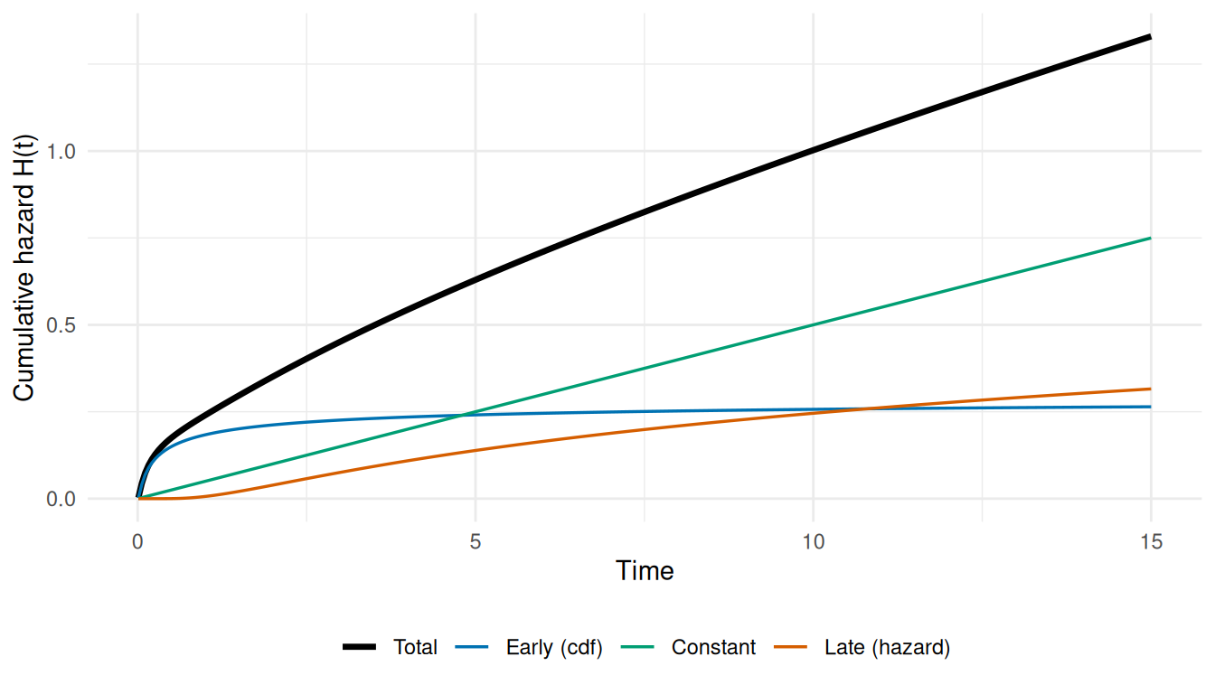
2.4 Additive composition example

To build intuition, here is how three phases combine into a total hazard. The key insight is that phases contribute additively to the cumulative hazard $H(t)$, not to the survival directly.

if (has_ggplot) {
  t_grid <- seq(0.01, 15, length.out = 300)

  mu_early <- 0.3
  mu_const <- 0.05
  mu_late  <- 0.2

  H_early <- mu_early * hzr_phase_cumhaz(t_grid, t_half = 0.5, nu = 2,
                                           m = 0, type = "cdf")
  H_const <- mu_const * hzr_phase_cumhaz(t_grid, type = "constant")
  H_late  <- mu_late  * hzr_phase_cumhaz(t_grid, t_half = 5, nu = 1,
                                           m = 0, type = "hazard")
  H_total <- H_early + H_const + H_late

  df <- data.frame(
    time = rep(t_grid, 4),
    cumhaz = c(H_early, H_const, H_late, H_total),
    component = rep(c("Early (cdf)", "Constant", "Late (hazard)", "Total"),
                    each = length(t_grid))
  )
  df$component <- factor(df$component,
    levels = c("Total", "Early (cdf)", "Constant", "Late (hazard)"))

  ggplot(df, aes(x = time, y = cumhaz, colour = component,
                 linewidth = component)) +
    geom_line() +
    scale_colour_manual(values = c(
      "Total" = "black", "Early (cdf)" = "#0072B2",
      "Constant" = "#009E73", "Late (hazard)" = "#D55E00"
    )) +
    scale_linewidth_manual(values = c(
      "Total" = 1.2, "Early (cdf)" = 0.6,
      "Constant" = 0.6, "Late (hazard)" = 0.6
    )) +
    labs(x = "Time", y = "Cumulative hazard H(t)",
         colour = NULL, linewidth = NULL) +
    theme_minimal(base_size = 11) +
    theme(legend.position = "bottom")
}

Figure 3: Three-phase additive cumulative hazard: total = early + constant + late

3 Maximum Likelihood Estimation

3.1 Log-likelihood under mixed censoring

TemporalHazard supports four censoring types in a single dataset, coded by the status indicator:

Code	Type	Contribution to log-likelihood
$\delta_i = 1$	Exact event	$\log h(t_i \mid \mathbf{x}_i) - H(t_i \mid \mathbf{x}_i)$
$\delta_i = 0$	Right-censored	$-H(t_i \mid \mathbf{x}_i)$
$\delta_i = -1$	Left-censored	$\log\bigl(1 - \exp(-H(u_i \mid \mathbf{x}_i))\bigr)$
$\delta_i = 2$	Interval-censored	$-H(l_i \mid \mathbf{x}_i) + \log\bigl(1 - \exp(-(H(u_i) - H(l_i)))\bigr)$

where $l_i$ and $u_i$ are the lower and upper bounds of the censoring interval.

The full log-likelihood is:

$$\ell(\boldsymbol{\theta}) = \sum_{i:\,\delta_i=1} \Bigl[\log h(t_i \mid \mathbf{x}_i) - H(t_i \mid \mathbf{x}_i)\Bigr] - \sum_{i:\,\delta_i=0} H(t_i \mid \mathbf{x}_i)$$$$+ \sum_{i:\,\delta_i=-1} \log\!\bigl(1 - e^{-H(u_i \mid \mathbf{x}_i)}\bigr) + \sum_{i:\,\delta_i=2} \Bigl[-H(l_i \mid \mathbf{x}_i) + \log\!\bigl(1 - e^{-(H(u_i) - H(l_i))}\bigr)\Bigr]$$

The $\log(1 - e^{-x})$ terms are computed using the numerically stable primitive hzr_log1mexp(), which avoids catastrophic cancellation when $x$ is near zero.

# Naive log(1 - exp(-x)) fails near zero
x_small <- 1e-15
cat("Naive:  ", log(1 - exp(-x_small)), "\n")
#> Naive:   -34.53958
cat("Stable: ", hzr_log1mexp(x_small), "\n")
#> Stable:  -34.53878

3.2 Internal parameterization

During optimization, shape parameters are reparameterized for unconstrained search. For each phase $j$, the internal parameter sub-vector is:

Parameter	Internal (estimation)	User-facing (reported)
Scale	$\log \mu_j$	$\mu_j = \exp(\log \mu_j)$
Half-life	$\log t_{1/2,j}$	$t_{1/2,j} = \exp(\log t_{1/2,j})$
Time exponent	$\nu_j$ (unconstrained)	$\nu_j$
Shape	$m_j$ (unconstrained)	$m_j$
Covariates	$\beta_{j,1}, \ldots, \beta_{j,p_j}$	same

Constant phases omit log_t_half, nu, and m, contributing only one shape-free parameter (log_mu). The full $\boldsymbol{\theta}$ is the concatenation of all phase sub-vectors.

3.3 Optimization strategy

The optimizer uses stats::optim() with BFGS on the unconstrained internal scale, wrapped by .hzr_optim_generic(). Key features:

• Multi-start: the optimizer runs from $k$ random perturbations around the user-supplied starting values (default $k = 5$, controlled by control$n_starts). The run with the highest log-likelihood is kept.
• Feasibility guard: any parameter vector where $m < 0$and $\nu < 0$ for the same phase returns $-\infty$ immediately.
• Post-fit Hessian: the numerical Hessian at the solution is inverted to produce the variance-covariance matrix. Standard errors are $\sqrt{\text{diag}(\hat{V})}$.

4 Covariates and Phase-Specific Formulas

4.1 Global covariates

By default, every phase shares the same covariate vector from the model formula. Each phase gets its own coefficient vector $\boldsymbol{\beta}_j$:

$$\mu_j(\mathbf{x}) = \exp\!\bigl(\alpha_j + \mathbf{x}\,\boldsymbol{\beta}_j\bigr)$$

This means the same predictors can have different effects on early vs. late risk — a core feature of multiphase models.

# Both phases use age and nyha from the global formula
hazard(
  survival::Surv(time, status) ~ age + nyha,
  data   = dat,
  dist   = "multiphase",
  phases = list(
    early = hzr_phase("cdf",    t_half = 0.5, nu = 2, m = 0),
    late  = hzr_phase("hazard", t_half = 5,   nu = 1, m = 0)
  ),
  fit = TRUE
)

4.2 Phase-specific covariates

When different phases are driven by different risk factors, each phase can specify its own one-sided formula:

# Early risk depends on surgical factors; late risk on chronic conditions
hazard(
  survival::Surv(time, status) ~ age + nyha + shock,
  data   = dat,
  dist   = "multiphase",
  phases = list(
    early = hzr_phase("cdf",    t_half = 0.5, nu = 2, m = 0,
                      formula = ~ age + shock),
    late  = hzr_phase("hazard", t_half = 5,   nu = 1, m = 0,
                      formula = ~ age + nyha)
  ),
  fit = TRUE
)

When a phase has a formula, it gets its own design matrix built from the data, and only those covariates appear in its $\boldsymbol{\beta}_j$. The parameter vector is shorter for phases with fewer covariates, which can improve identifiability and convergence.

4.3 Time-varying coefficients

For single-distribution models, TemporalHazard supports piecewise time-varying coefficients via the time_windows argument. This expands the design matrix into window-specific blocks:

$$\eta_i = \sum_{k=1}^{K} \mathbf{x}_i \boldsymbol{\beta}_k \cdot \mathbf{1}(t_i \in W_k)$$

where $W_1, \ldots, W_K$ are the time windows defined by the cut points. Each predictor gets a separate coefficient in each window, allowing effects to change over follow-up time.

# Two windows: [0, 2] and (2, infinity)
hazard(
  survival::Surv(time, status) ~ age + nyha,
  data         = dat,
  theta        = c(mu = 0.25, nu = 1.1,
                   age_w1 = 0, nyha_w1 = 0,
                   age_w2 = 0, nyha_w2 = 0),
  dist         = "weibull",
  time_windows = 2,
  fit          = TRUE
)

Multiphase vs. time-varying coefficients

For multiphase models, the phase structure itself captures time-varying effects: early phases dominate at small $t$ and late phases at large $t$. The time_windows mechanism is a complementary approach for single-distribution models.

5 Identifiability and Practical Considerations

5.1 Parameter identifiability

Multiphase models with many free parameters can have flat or multi-modal likelihood surfaces. Practical guidelines:

1. Fix shape parameters when possible. If clinical knowledge suggests a specific temporal pattern (e.g. early mortality follows a Weibull shape with $m = 0$), fix m in the hzr_phase() starting values and inspect whether the optimizer moves it.

2. Start from the SAS/C estimates. If legacy results are available, translate them using hzr_argument_mapping() and supply as starting values.

3. Use multi-start optimization. The default control$n_starts = 5 helps escape local optima, but complex models may benefit from more starts.

4. Phase-specific covariates improve identifiability. Restricting each phase to clinically relevant predictors reduces the parameter count and sharpens the likelihood surface.

5.2 Numerical stability

The decomposition engine applies several guards:

• Time is clamped above .Machine$double.xmin to avoid $0^{\text{negative}}$
• $1 - G(t)$ is clamped above .Machine$double.xmin before computing the hazard $h(t) = g(t)/(1 - G(t))$
• Left- and interval-censored contributions use hzr_log1mexp() to avoid $\log(0)$ when $H(t)$ is very small

These guards ensure finite gradients throughout the optimization, even in regions of parameter space far from the optimum.

6 Summary of Key Functions

Function	Purpose
hzr_decompos(t, t_half, nu, m)	Core decomposition: returns $G$, $g$, $h$
hzr_phase_cumhaz(t, ..., type)	Phase cumulative hazard $\Phi(t)$
hzr_phase_hazard(t, ..., type)	Phase instantaneous hazard $\varphi(t)$
hzr_phase(type, t_half, nu, m, formula)	Construct a phase specification
hazard(..., dist = "multiphase", phases = ...)	Fit a multiphase model
predict(fit, type, decompose = TRUE)	Per-phase decomposed predictions
hzr_argument_mapping()	SAS/C $\to$ R parameter translation table
hzr_log1mexp(x)	Stable $\log(1 - e^{-x})$

For a worked clinical example, see vignette("getting-started"). For migration from SAS HAZARD, see vignette("sas-to-r-migration").

References

Blackstone EH, Naftel DC, Turner ME Jr. The decomposition of time-varying hazard into phases, each incorporating a separate stream of concomitant information. J Am Stat Assoc. 1986;81(395):615–624. doi: 10.1080/01621459.1986.10478314

Rajeswaran J, Blackstone EH, Ehrlinger J, Li L, Ishwaran H, Parides MK. Probability of atrial fibrillation after ablation: Using a parametric nonlinear temporal decomposition mixed effects model. Stat Methods Med Res. 2018;27(1):126–141. doi: 10.1177/0962280215623583