Inference & Diagnostics
Exploratory screening, bootstrap confidence intervals, and sensitivity analysis
Source:vignettes/inference-diagnostics.qmd
Fitting a hazard model is the middle of the workflow, not the end. Before you fit, you screen the covariates so you know what transformations the data actually supports. After you fit, you quantify uncertainty (bootstrap CIs, Wald intervals), check whether the model is honest to the data (goodness-of-fit overlays, decile-of-risk calibration), and probe its behavior under different covariate scenarios (sensitivity analysis). This vignette walks the diagnostic and inferential tools the package ships for each of those steps.
These pieces correspond directly to steps in the classic SAS HAZARD workflow — the lg.* logistic-screening macros, the bs.* bootstrap macros, the hs.* hazard-sensitivity macros — re-implemented as first-class R functions (hzr_calibrate(), hzr_kaplan(), hzr_nelson(), hzr_bootstrap(), hzr_gof(), hzr_deciles()). If you’ve worked through a SAS HAZARD analysis you already know the shape of what follows; if not, treat this vignette as the standard diagnostic pass you’d run on any fitted hazard model before trusting its conclusions.
1 Exploratory covariate screening
Before fitting the parametric hazard model, screen each candidate covariate with a simple logistic regression against the event indicator. This is much cheaper than fitting the full hazard model and answers two distinct questions: which covariates carry signal at all (rough significance triage), and what functional form each covariate enters with — linear, log, polynomial, or something non-monotone that needs binning. The screening step is what stops you from blindly throwing every column at hazard() and then trying to debug a model that has shape mis-specification baked in.
Fit a univariable logistic regression for each candidate against the death indicator. The p-values that come out are not the final word on whether a covariate matters — they ignore the joint structure of the hazard model and they treat the event time as a binary outcome — but they do tell you which covariates have no chance of mattering, and which deserve closer inspection.
logit_fits <- lapply(candidates, function(var) {
  fmla <- as.formula(paste("dead ~", var))
  glm(fmla, data = avc, family = binomial())
})
names(logit_fits) <- candidates

# Which covariates are significant univariably?
p_values <- vapply(logit_fits, function(f) {
  coef(summary(f))[2, "Pr(>|z|)"]
}, numeric(1))

data.frame(covariate = names(p_values),
           p_value   = round(p_values, 4),
           row.names = NULL)
#>   covariate p_value
#> 1       age  0.0017
#> 2    status  0.0000
#> 3       mal  0.0006
#> 4    com_iv  0.0000
#> 5  inc_surg  0.0114
#> 6   orifice  0.0034
ggplot(avc, aes(age, dead)) +
  geom_jitter(height = 0.05, width = 0, alpha = 0.3, size = 1) +
  geom_smooth(method = "loess", se = TRUE, colour = "#0072B2",
              linewidth = 0.8) +
  labs(x = "Age at operation (months)", y = "Death (0/1)") +
  theme_minimal()
#> `geom_smooth()` using formula = 'y ~ x'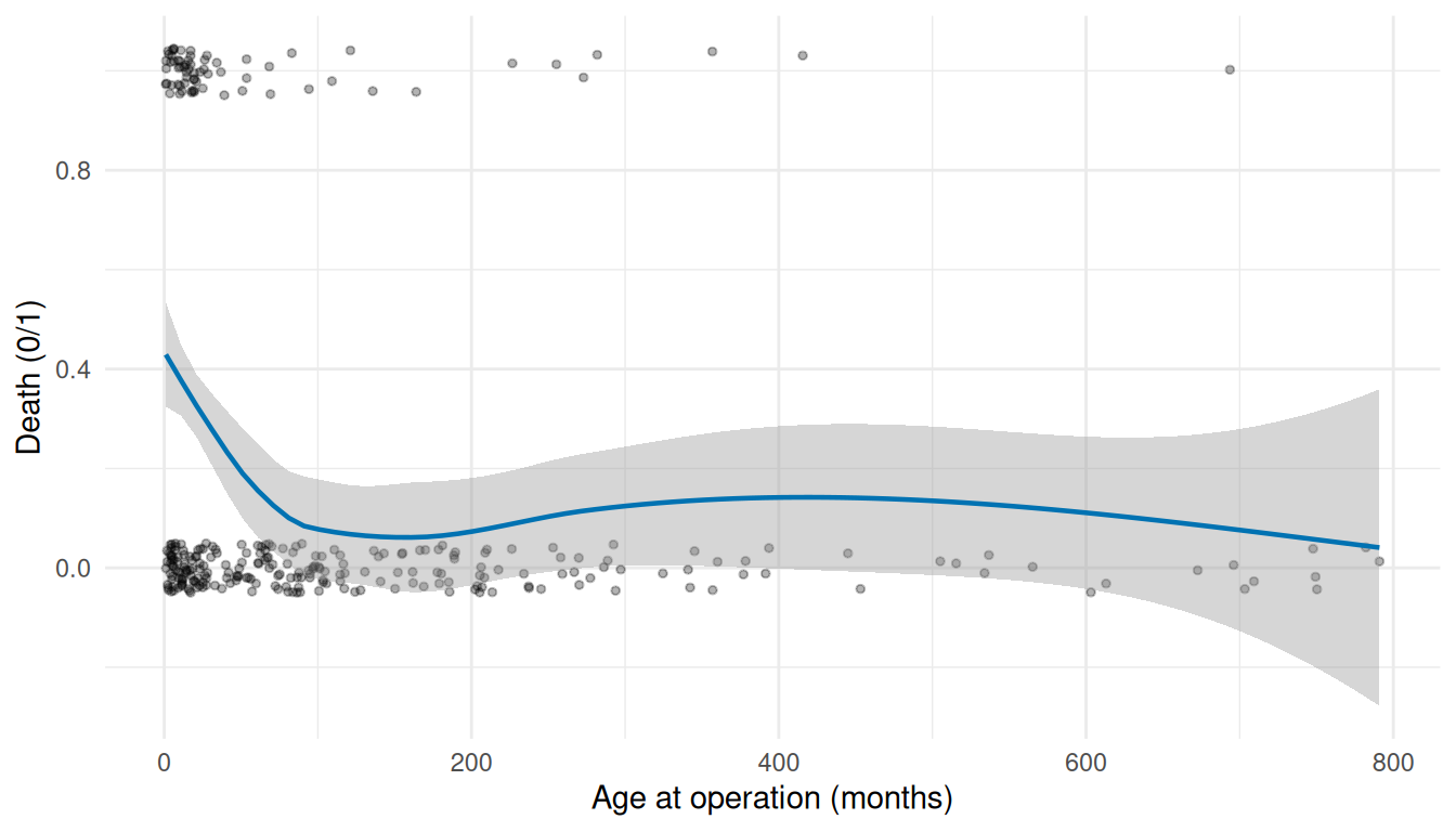
The LOESS smooth reveals the shape of the covariate-mortality relationship in a non-parametric way. A roughly linear smooth means the covariate enters the hazard model on its natural scale; a U or inverted-U shape means a polynomial or a non-monotone transform; a plateau-then-rise means a threshold effect that may need binning. This is the call you make before writing the formula for hazard(), not after staring at a converged-but-misspecified model.
1.1 Quantile calibration with hzr_calibrate()
hzr_calibrate() bins a continuous covariate into quantile groups and applies the logit / Gompertz / Cox link transform, so you can eyeball whether the covariate-outcome relationship is linear on the chosen link scale. It corresponds to the SAS logit.sas / logitgr.sas macros.
age_cal <- hzr_calibrate(
  x      = avc$age,
  event  = avc$dead,
  groups = 10,
  link   = "logit"
)
print(age_cal)
#> Variable calibration (logit link, 10 groups)
#>
#>  group  n events    mean     min     max  prob link_value
#>      1 30     11   3.519   1.051   5.388 0.367     -0.547
#>      2 31     11   8.665   5.421  11.532 0.355     -0.598
#>      3 30     13  15.194  11.631  18.497 0.433     -0.268
#>      4 31     11  23.077  18.990  27.828 0.355     -0.598
#>      5 30      7  43.544  28.124  57.167 0.233     -1.190
#>      6 31      3  72.066  59.730  86.408 0.097     -2.234
#>      7 30      2 101.154  86.507 117.522 0.067     -2.639
#>      8 31      3 162.739 121.169 203.733 0.097     -2.234
#>      9 30      4 247.051 205.343 297.140 0.133     -1.872
#>     10 31      3 530.623 324.573 790.981 0.097     -2.234
A roughly linear trend across groups means the logit link is appropriate; strong curvature flags the need for a transform (for example, polynomial or log).
2 Nonparametric baselines
A parametric fit has to be compared against something. The natural something is the nonparametric estimate of the same quantity from the same data — Kaplan-Meier for survival, Nelson-Aalen for cumulative hazard. The package’s hzr_kaplan() and hzr_nelson() are convenience wrappers that return richer output than survival::survfit(): hzr_kaplan() ships KM with logit-transformed confidence limits (more accurate in the tails than the standard Greenwood limits, which can stray outside \([0, 1]\)), interval hazard rates, density estimates, and a restricted-mean-survival-time scalar. hzr_nelson() returns the Wayne Nelson cumulative hazard estimator with log-normal confidence limits — the right reference when you care about the integrated intensity rather than the survival probability.
km <- hzr_kaplan(time = avc$int_dead, status = avc$dead, conf_level = 0.95)
print(km)
#> Kaplan-Meier estimate with logit confidence limits
#> Events: 68  | Time points: 44
#> Survival range: 0 to 0.9836
#> RMST at last event: 129.3468
#>
#>         time n_risk n_event n_censor survival std_err cl_lower cl_upper cumhaz
#>  0.001368954    305       5        0   0.9836  0.0073   0.9612   0.9932 0.0165
#>  0.002737907    300       2        0   0.9770  0.0086   0.9527   0.9890 0.0232
#>  0.008213721    298       2        0   0.9705  0.0097   0.9443   0.9846 0.0300
#>  0.016427440    296       5        0   0.9541  0.0120   0.9240   0.9726 0.0470
#>  0.032854880    291       3        0   0.9443  0.0131   0.9122   0.9651 0.0574
#>  0.049282330    288       1        0   0.9410  0.0135   0.9083   0.9625 0.0608
#>  0.053389190    287       1        0   0.9377  0.0138   0.9044   0.9599 0.0643
#>  0.054758140    286       1        0   0.9344  0.0142   0.9006   0.9573 0.0678
#>  0.065709770    285       5        0   0.9180  0.0157   0.8815   0.9440 0.0855
#>  0.071185580    280       1        0   0.9148  0.0160   0.8777   0.9413 0.0891
#>  0.082137210    279       2        0   0.9082  0.0165   0.8702   0.9359 0.0963
#>  0.098564650    277       2        0   0.9016  0.0171   0.8628   0.9304 0.1035
#>  0.114992100    275       3        0   0.8918  0.0178   0.8517   0.9221 0.1145
#>  0.131419500    272       1        0   0.8885  0.0180   0.8480   0.9193 0.1182
#>  0.229984200    270       2        0   0.8819  0.0185   0.8407   0.9136 0.1256
#>  0.262839100    268       1        1   0.8787  0.0187   0.8370   0.9108 0.1294
#>  0.279266500    266       1        0   0.8753  0.0189   0.8333   0.9080 0.1331
#>  0.328548800    264       2        0   0.8687  0.0194   0.8259   0.9022 0.1407
#>  0.344976300    262       1        0   0.8654  0.0196   0.8223   0.8993 0.1446
#>  0.377831200    261       1        0   0.8621  0.0198   0.8186   0.8965 0.1484
#>   hazard density   life
#>  12.0744 11.9752 0.0014
#>   4.8862  4.7901 0.0027
#>   1.2298  1.1975 0.0081
#>   2.0741  1.9959 0.0160
#>   0.6308  0.5988 0.0317
#>   0.2117  0.1996 0.0472
#>   0.8499  0.7983 0.0511
#>   2.5586  2.3950 0.0524
#>   1.6162  1.4969 0.0626
#>   0.6534  0.5988 0.0676
#>   0.6569  0.5988 0.0776
#>   0.4411  0.3992 0.0926
#>   0.6677  0.5988 0.1074
#>   0.2242  0.1996 0.1220
#>   0.2263  0.2003 0.2096
#>   0.1138  0.1002 0.2386
#>   0.2293  0.2011 0.2530
#>   0.2315  0.2018 0.2962
#>   0.2328  0.2018 0.3104
#>   0.1168  0.1009 0.3389
#> ... ( 24  more rows)
nel <- hzr_nelson(time = avc$int_dead, event = avc$dead, conf_level = 0.95)
print(nel)
#> Nelson cumulative hazard estimate with lognormal CL
#> Events: 68  | Time points: 44
#>
#>         time n_risk n_event weight_sum cumhaz std_err cl_lower cl_upper  hazard
#>  0.001368954    305       5          5 0.0164  0.0033   0.0109   0.0237 11.9752
#>  0.002737907    300       2          2 0.0231  0.0047   0.0153   0.0335  4.8699
#>  0.008213721    298       2          2 0.0298  0.0057   0.0201   0.0425  1.2256
#>  0.016427440    296       5          5 0.0467  0.0067   0.0350   0.0610  2.0565
#>  0.032854880    291       3          3 0.0570  0.0075   0.0437   0.0730  0.6276
#>  0.049282330    288       1          1 0.0604  0.0082   0.0459   0.0782  0.2114
#>  0.053389190    287       1          1 0.0639  0.0089   0.0482   0.0832  0.8484
#>  0.054758140    286       1          1 0.0674  0.0096   0.0506   0.0881  2.5541
#>  0.065709770    285       5          5 0.0850  0.0102   0.0667   0.1067  1.6019
#>  0.071185580    280       1          1 0.0885  0.0108   0.0692   0.1116  0.6522
#>  0.082137210    279       2          2 0.0957  0.0114   0.0753   0.1199  0.6546
#>  0.098564650    277       2          2 0.1029  0.0119   0.0815   0.1282  0.4395
#>  0.114992100    275       3          3 0.1138  0.0125   0.0913   0.1402  0.6641
#>  0.131419500    272       1          1 0.1175  0.0130   0.0941   0.1450  0.2238
#>  0.229984200    270       2          2 0.1249  0.0135   0.1006   0.1534  0.0752
#>  0.262839100    268       1          1 0.1287  0.0140   0.1034   0.1582  0.1136
#>  0.279266500    266       1          1 0.1324  0.0145   0.1063   0.1629  0.2288
#>  0.328548800    264       2          2 0.1400  0.0149   0.1130   0.1715  0.1537
#>  0.344976300    262       1          1 0.1438  0.0154   0.1160   0.1763  0.2323
#>  0.377831200    261       1          1 0.1476  0.0158   0.1190   0.1811  0.1166
#>  cum_events
#>           5
#>           7
#>           9
#>          14
#>          17
#>          18
#>          19
#>          20
#>          25
#>          26
#>          28
#>          30
#>          33
#>          34
#>          36
#>          37
#>          38
#>          40
#>          41
#>          42
#> ... ( 24  more rows)
3 Bootstrap confidence intervals
The delta-method CIs predict(se.fit = TRUE) returns are fast and asymptotically correct, but they lean on the Hessian-derived parameter vcov — which can mislead when the likelihood surface is poorly behaved near the MLE (boundary fits, near-degenerate parameter combinations, small samples). The package flags these cases for you: each fit carries rcond and pd diagnostics, and summary() prints a note (with a matching warning at fit time) when the Hessian is ill-conditioned or not positive-definite — a strong signal to prefer the bootstrap. Bootstrap resampling is the robust alternative: refit the model on each resampled dataset, collect the resulting parameter and prediction values, and read the empirical 2.5th / 97.5th percentiles as the 95% CI. It’s computationally heavier but it doesn’t assume the likelihood is locally quadratic, and it picks up the right tail behavior even when delta-method theory creaks.
hzr_bootstrap() wraps the resample-and-refit loop and corresponds to the SAS bootstrap.hazard.sas and bootstrap.summary.sas macros. We fit a base model first; bootstrap replicates will resample from the same data and refit using these starting values.
# Fit the base model that bootstrapping will use
fit <- hazard(
  Surv(int_dead, dead) ~ age + status + mal + com_iv,
  data  = avc,
  dist  = "weibull",
  theta = c(mu = 0.20, nu = 1.0, rep(0, 4)),
  fit   = TRUE,
  control = list(maxit = 500)
)

# Prediction grid at a median-risk profile
t_grid <- seq(0.01, max(avc$int_dead) * 0.9, length.out = 100)
base_nd <- data.frame(time = t_grid, age = median(avc$age),
                      status = 2, mal = 0, com_iv = 0)

surv_point <- predict(fit, newdata = base_nd, type = "survival")
hzr_bootstrap() returns a long data frame of per-replicate coefficient estimates ($replicates) and a parameter-level summary (mean, SD, 95% percentile CI) in $summary. We use n_boot = 30 here purely so the vignette renders in reasonable time — for a real analysis you’d want 200 or more replicates. The set.seed(42) call before hzr_bootstrap() makes the resample sequence reproducible.
set.seed(42)
boot <- hzr_bootstrap(fit, n_boot = 30)  # kept small for vignette build time
print(boot)
#> Bootstrap inference for hazard model
#> Mode: fixed refit
#> Replicates: 30 successful, 0 failed
#>
#>  parameter  n pct    mean     sd     min    max ci_lower ci_upper
#>         mu 30 100  0.0000 0.0000  0.0000 0.0000   0.0000   0.0000
#>         nu 30 100  0.2174 0.0603  0.0004 0.2668   0.0012   0.2587
#>        age 30 100 -0.0025 0.0024 -0.0100 0.0026  -0.0079   0.0011
#>     status 30 100  0.6778 0.1666  0.2712 1.0751   0.3792   0.9582
#>        mal 30 100  0.4165 0.3526 -0.4065 0.9703  -0.3595   0.9447
#>     com_iv 30 100  0.9099 0.4358  0.0609 2.0954   0.2661   2.0265
The parameter-level CIs above come directly from the bootstrap distribution. Prediction-level CIs (on the survival curve or hazard profile) require pivoting boot$replicates to wide format and evaluating the parametric survival formula once per replicate. That workflow is out of scope for this section, but the building blocks are all in the returned object.
4 Goodness-of-fit overlay
The Kaplan-Meier overlay in the prediction-visualization vignette is the visual goodness-of-fit check. hzr_gof() is the quantitative complement: it tabulates parametric predictions side by side with the nonparametric KM estimate at each event time, and computes the Conservation-of-Events observed-vs-expected ratio across the whole follow-up window. The ratio compresses everything the model is doing into a single number, which makes it the right summary statistic to report alongside coefficient tables. (hzr_gof() corresponds to the SAS hazplot.sas macro.)
gof <- hzr_gof(fit)
print(gof)
#> Goodness-of-fit: observed vs. expected events
#> Distribution: weibull  | n = 305
#>
#> Total observed events: 68
#> Total expected events: 50.433
#> Final residual (E - O): -17.567
#> Conservation ratio (E/O): 0.742
#>
#> Use plot columns: time, km_surv, par_surv, cum_observed, cum_expected, residual
The observed vs. expected ratio (printed at the bottom) is the Conservation-of-Events check: a well-specified model recovers the event count exactly, so a ratio close to 1 is what we want. Ratios well above or below 1 flag either a misspecified shape or a covariate that isn’t really linear on the log-hazard scale.
5 Decile-of-risk calibration
The conservation-of-events ratio above tells you whether the model is calibrated on average. That’s necessary but not sufficient — a model can hit the right total event count while systematically over-predicting risk for one part of the cohort and under-predicting for another, with the errors cancelling in aggregate. hzr_deciles() is the check that catches that failure mode: it partitions patients into deciles of predicted risk at a chosen time point and compares observed with expected event counts within each decile, returning a chi-square goodness-of-fit test. A well-calibrated model has observed-vs-expected close in every decile; a model that’s globally calibrated but locally biased will show large residuals in the extreme deciles. (Corresponds to the SAS deciles.hazard.sas macro.)
deciles <- hzr_deciles(fit, time = 120, groups = 10)
print(deciles)
#> Decile-of-risk calibration (risk grouped at time = 120 )
#> 305 subjects, all included.
#> 10 groups, 68 observed events, 68 expected
#>
#>  group  n events expected observed_rate expected_rate chi_sq p_value
#>      1 31      0     1.37        0.0000        0.0441 1.3700  0.2420
#>      2 30      1     1.64        0.0333        0.0546 0.2480  0.6190
#>      3 31      1     2.53        0.0323        0.0816 0.9250  0.3360
#>      4 30      2     3.49        0.0667        0.1160 0.6350  0.4260
#>      5 31      7     4.58        0.2260        0.1480 1.2800  0.2570
#>      6 30     10     5.67        0.3330        0.1890 3.3100  0.0689
#>      7 31      8     7.59        0.2580        0.2450 0.0218  0.8830
#>      8 30     14     8.71        0.4670        0.2900 3.2100  0.0734
#>      9 31     10    13.50        0.3230        0.4350 0.8960  0.3440
#>     10 30     15    18.90        0.5000        0.6320 0.8220  0.3650
#>  mean_survival mean_cumhaz
#>          0.950      0.0441
#>          0.931      0.0546
#>          0.906      0.0816
#>          0.865      0.1160
#>          0.818      0.1480
#>          0.708      0.1890
#>          0.655      0.2450
#>          0.538      0.2900
#>          0.441      0.4350
#>          0.221      0.6320
#>
#> Overall: chi-sq = 12.7 on 9 df, p = 0.176
The chi-square test statistic and p-value summarise whether the observed decile-by-decile event counts are consistent with what the parametric model predicts. A good visual check is to plot the two columns side by side:
decile_df <- as.data.frame(deciles)
cal_long <- rbind(
  data.frame(group = decile_df$group,
             rate  = decile_df$observed_rate,
             Series = "Observed"),
  data.frame(group = decile_df$group,
             rate  = decile_df$expected_rate,
             Series = "Expected")
)
ggplot(cal_long, aes(group, rate, fill = Series)) +
  geom_col(position = position_dodge(width = 0.7), alpha = 0.8) +
  scale_fill_manual(values = c("Observed" = "#56B4E9",
                                "Expected" = "#E69F00")) +
  scale_x_continuous(breaks = seq_len(nrow(decile_df))) +
  scale_y_continuous(labels = scales::percent_format(accuracy = 1)) +
  labs(x = "Risk decile (1 = lowest)", y = "Mortality rate", fill = NULL) +
  theme_minimal() +
  theme(legend.position = "bottom")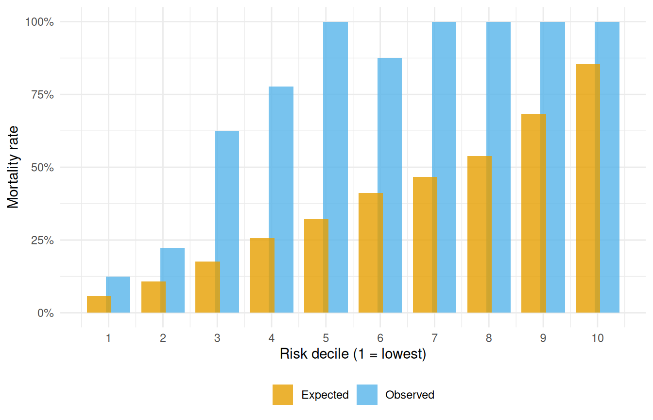
6 Sensitivity analysis
Coefficient estimates tell you the direction and magnitude of a covariate’s effect on the hazard scale, but they don’t directly answer the clinical question of what survival difference this implies for a real patient. Sensitivity analysis closes that gap. You define two or more covariate profiles — typically a reference profile and one or more high-risk profiles — score each through predict(), and plot the resulting survival curves on shared axes. The horizontal and vertical gaps between curves translate the model’s coefficients into the clinically meaningful currency of survival probability differences and median-survival shifts. It’s also a stress test: if your high-risk profile produces only a small survival gap, either the risk factors aren’t doing much in this cohort, or the model is missing the mechanism that makes them matter.
# Define reference and high-risk profiles
ref_profile <- data.frame(
  age    = median(avc$age),
  status = 2,
  mal    = 0,
  com_iv = 0
)

high_risk <- data.frame(
  age    = quantile(avc$age, 0.90),
  status = 4,
  mal    = 1,
  com_iv = 1
)
sens_curves <- do.call(rbind, lapply(
  list("Reference" = ref_profile, "High risk" = high_risk),
  function(p) {
    nd <- p[rep(1, length(t_grid)), ]
    nd$time <- t_grid
    data.frame(time = t_grid,
               survival = predict(fit, newdata = nd, type = "survival") * 100,
               Profile = deparse(substitute(p)))
  }
))
# Fix profile labels
sens_curves$Profile <- rep(c("Reference", "High risk"),
                           each = length(t_grid))
sens_curves$Profile <- factor(sens_curves$Profile,
                              levels = c("Reference", "High risk"))

ggplot(sens_curves, aes(time, survival, colour = Profile)) +
  geom_line(linewidth = 0.9) +
  scale_colour_manual(values = c("Reference" = "#009E73",
                                 "High risk" = "#D55E00")) +
  scale_y_continuous(limits = c(0, 100)) +
  labs(x = "Months after AVC repair", y = "Freedom from death (%)",
       colour = NULL) +
  theme_minimal() +
  theme(legend.position = "bottom")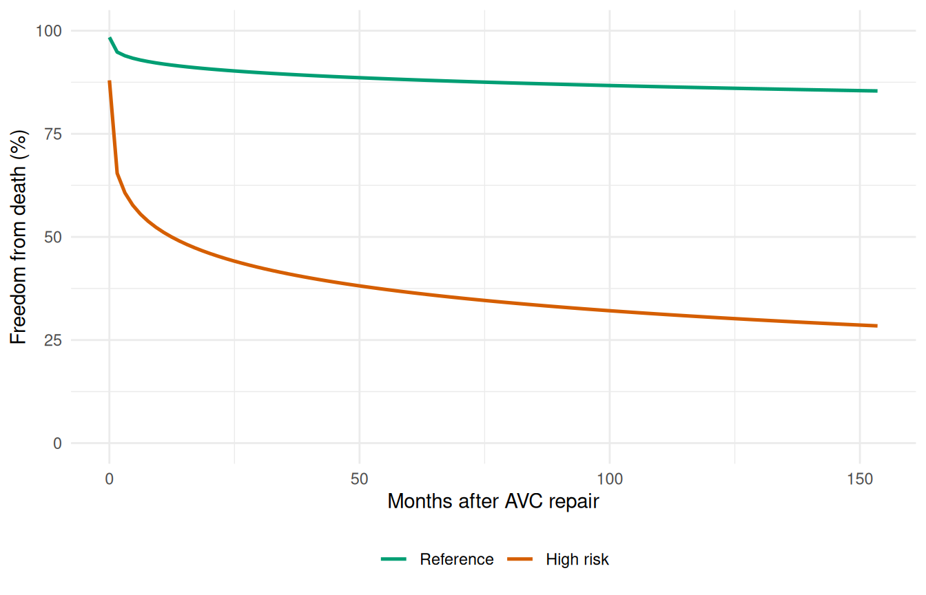
The gap between the curves quantifies the clinical impact of the risk factors. The sensitivity analysis is most informative when combined with bootstrap confidence intervals on each curve, showing whether the difference is statistically meaningful.
7 Analysis workflow summary
The pieces in this vignette aren’t independent diagnostics — they chain together into a single analytical workflow that goes from raw covariates to a defensible, uncertainty-quantified, well-calibrated fitted model. The complete sequence, with the SAS HAZARD correspondences each piece descends from:
-
Exploratory screening (
glm,hzr_calibrate()) — identify covariate transformations and functional forms -
Nonparametric baselines (
hzr_kaplan(),hzr_nelson()) — reference KM / Nelson cumulative hazard estimators -
Fit hazard model (
hazard()) — parametric shape + covariates -
Predict & visualize (
predict()) — survival, hazard, risk profiles -
Goodness-of-fit overlay (
hzr_gof()) — parametric vs. KM + Conservation-of-Events check -
Bootstrap CIs (
hzr_bootstrap()) — uncertainty quantification via resampling -
Sensitivity analysis (
predict()on covariate profiles) — compare scenarios across risk factors -
Decile calibration (
hzr_deciles()) — chi-square observed vs. expected by risk decile
See vignette("getting-started") for the minimal workflow and vignette("fitting-hazard-models") for the model-fitting details.