Kaplan-Meier survival with exact logit confidence limits

Compute the product-limit (Kaplan-Meier) survival estimate with logit-transformed confidence limits that respect the $[0, 1]$ boundary. This is the R equivalent of the SAS kaplan.sas macro.

Usage

hzr_kaplan(time, status, conf_level = 0.95, event_only = TRUE)

Arguments

time: Numeric vector of follow-up times.
status: Numeric event indicator (1 = event, 0 = censored).
conf_level: Confidence level for the interval (default 0.95). The SAS default of 0.68268948 corresponds to a 1-SD interval.
event_only: Logical; if TRUE (default), only return rows at event times (where n_event > 0). If FALSE, return rows at all times reported by survival::survfit() (events and censoring times).

Value

A data frame with one row per time point and columns:

time: Event/censoring time.
n_risk: Number at risk at start of interval.
n_event: Number of events at this time.
n_censor: Number censored at this time.
survival: Kaplan-Meier survival estimate.
std_err: Standard error of survival (Greenwood).
cl_lower: Lower confidence limit (logit-transformed).
cl_upper: Upper confidence limit (logit-transformed).
cumhaz: Cumulative hazard $= -\log(S)$.
hazard: Interval hazard rate $= \log(S_{t-1} / S_t) / \Delta t$.
density: Probability density estimate $= (S_{t-1} - S_t) / \Delta t$.
life: Restricted mean survival time (area under curve to this time).

Details

The standard Greenwood confidence interval can exceed $[0, 1]$ in the tails. The logit-transformed interval avoids this by working on the log-odds scale:

$$ \text{CL}_{\text{lower}} = S / \bigl(S + (1-S)\, \exp(z_\alpha\,\text{SI})\bigr) $$ $$ \text{CL}_{\text{upper}} = S / \bigl(S + (1-S)\, \exp(-z_\alpha\,\text{SI})\bigr) $$

where $\text{SI} = \sqrt{V_P - 1} / (1 - S)$, $V_P$ is the cumulative Greenwood variance product, and $z_\alpha$ is the normal quantile for the requested confidence level.

Examples

data(cabgkul)
km <- hzr_kaplan(cabgkul$int_dead, cabgkul$dead)
head(km)
#> Kaplan-Meier estimate with logit confidence limits
#> Events: 69  | Time points: 6 
#> Survival range: 0.9883 to 0.9934 
#> RMST at last event: 0.1957 
#> 
#>     time n_risk n_event n_censor survival std_err cl_lower cl_upper cumhaz
#>  0.03285   5880      39        0   0.9934  0.0011   0.9909   0.9952 0.0067
#>  0.06571   5841       9        0   0.9918  0.0012   0.9892   0.9938 0.0082
#>  0.09856   5832       3        0   0.9913  0.0012   0.9886   0.9934 0.0087
#>  0.13142   5829       7        0   0.9901  0.0013   0.9873   0.9924 0.0099
#>  0.16427   5822       9        0   0.9886  0.0014   0.9855   0.9910 0.0115
#>  0.19713   5813       2        0   0.9883  0.0014   0.9852   0.9907 0.0118
#>  hazard density   life
#>  0.2026  0.2019 0.0328
#>  0.0469  0.0466 0.0655
#>  0.0157  0.0155 0.0981
#>  0.0366  0.0362 0.1306
#>  0.0471  0.0466 0.1632
#>  0.0105  0.0104 0.1957

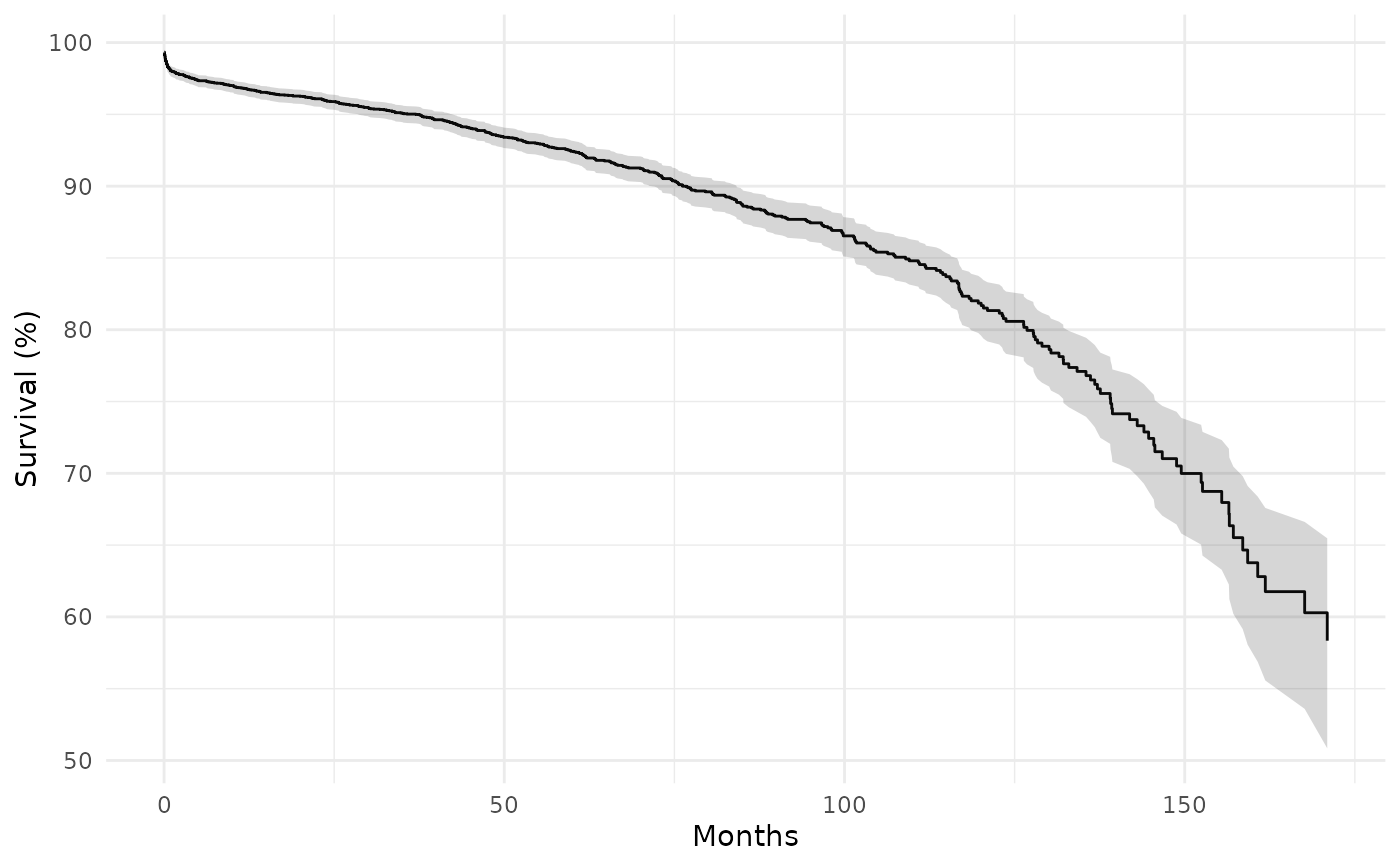
# \donttest{
if (requireNamespace("ggplot2", quietly = TRUE)) {
  library(ggplot2)
  ggplot(km, aes(time)) +
    geom_step(aes(y = survival * 100)) +
    geom_ribbon(aes(ymin = cl_lower * 100, ymax = cl_upper * 100),
                stat = "identity", alpha = 0.2) +
    labs(x = "Months", y = "Survival (%)") +
    theme_minimal()
}

# }

References

Kaplan EL, Meier P (1958). Nonparametric estimation from incomplete observations. J Am Stat Assoc 53(282):457–481. doi:10.1080/01621459.1958.10501452
Greenwood M (1926). The natural duration of cancer. Reports on Public Health and Medical Subjects 33:1–26.
See also
hzr_gof() for parametric vs. nonparametric comparison.