Per-variable lasso-beta importance from a varPro fit

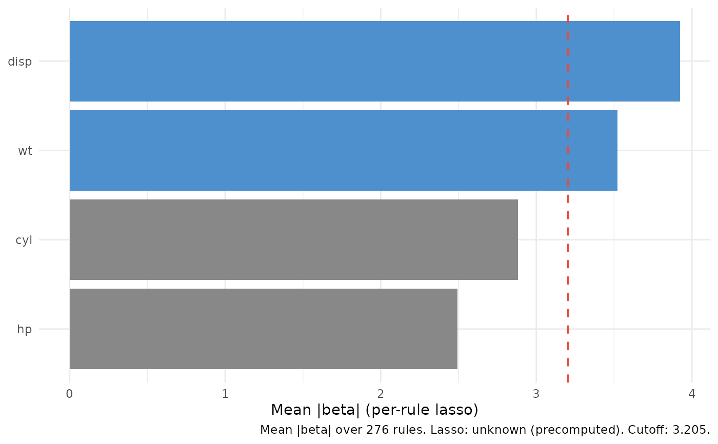
Tidy wrapper around varPro::beta.varpro() for the regression or classification family. Aggregates the per-rule lasso coefficient $\hat{\beta}$ by variable into the mean absolute value $\mathrm{mean}(|\hat{\beta}|)$ and flags variables above a scalar cutoff. Optional beta_fit argument lets callers compute the expensive beta.varpro() step once and reuse the result.

Usage

gg_beta_varpro(object, ..., cutoff = NULL, beta_fit = NULL, which_class = NULL)

Arguments

object: A varpro fit from varPro::varpro() (regression or classification family).
...: Forwarded to varPro::beta.varpro() when beta_fit = NULL; ignored otherwise (with a warning). Documented forwardables: use.cv, use.1se, nfolds, maxit, thresh, max.rules.tree, max.tree.
cutoff: Selection threshold on beta_mean. NULL (default) means mean(beta_mean) across released variables. Numeric scalar otherwise.
beta_fit: Optional pre-computed varPro::beta.varpro() result for the same object. NULL (default) means the wrapper runs beta.varpro() itself. When supplied, must be a varpro-class object whose $results has columns tree / branch / variable / n.oob / imp.
which_class: For a classification fit, name of a single response level to subset on. NULL (default) returns all classes (binary fits resolve to the last factor level, the positive-class convention used by glm and gg_roc). Ignored with a warning on regression fits.

Value

A data.frame of class c("gg_beta_varpro", "data.frame"). For a regression fit: one row per released variable, sorted by beta_mean descending. For a classification fit: long-format with an extra class column, one row per (variable, class) pair; variable is a factor whose levels are set by mean(|sum-of-class-beta|) descending so every facet / panel shares the same row order. which_class (or the binary default last-factor-level) collapses the output to a single class.

Note

Multivariate regression (regr+) and survival families are out of scope for this release and tracked for v3.1.0. The unsupported-family path errors with a message pointing at that work.

What this is doing

Think of the varPro release-rule mechanism as asking: "given a region of the feature space that the forest carved out, what changes when I remove the constraint on this one variable and let observations leave?" The standard importance answer (from gg_varpro()) measures that change as a z-scored contrast between local estimators: no synthetic data, no permutation. beta.varpro() asks the same question with a different ruler: for each rule (a tree-branch pair), it fits a one-predictor lasso regression of the response on the released variable's values, restricted to the OOB observations inside the rule's region. The wrapper aggregates those per-rule coefficients into one number per variable.

The key distinction from gg_vimp(), which measures Breiman-Cutler permutation importance by perturbing a variable's values and watching OOB error climb, is that neither gg_varpro() nor gg_beta_varpro() touches the data synthetically: all contrasts are between real subsets defined by the forest's rules.

What `imp` actually is (pedantic, because the column name is misleading)

The imp column on beta.varpro()'s $results is not a variable-importance score in the conventional sense. It is a regularised regression coefficient. Specifically:

Per rule, glmnet fits a one-predictor lasso of the response on the released variable inside the rule's OOB region. use.cv = TRUE selects $\lambda$ by 10-fold CV (default nfolds = 10); use.1se = TRUE (default) picks lambda.1se. use.cv = FALSE uses the full $\lambda$ path.
imp is the fitted coefficient $\hat{\beta}$ at the chosen $\lambda$. Sign is real (direction of local association). Magnitude depends on the predictor's units (raw x, no standardisation); a predictor in millimetres has a smaller $|\hat{\beta}|$ than the same predictor in metres.
Lasso shrinkage can drive $\hat{\beta}$ to exactly zero. Those zeros are data, not missingness, and are kept in the aggregation. Convergence failures land as NA_real_ and are dropped.
The per-variable aggregate is beta_mean, $\mathrm{mean}(|\hat{\beta}|)$, across the rules where this variable was released. It is not a permutation importance, not a split-strength importance, and not directly comparable on the same numeric axis to gg_varpro()'s z-scores. Disagreement with gg_varpro is often diagnostic, not a bug.

In code form: imp_r is the glmnet coefficient $\hat{\beta}$ fit on y ~ x_v restricted to rule r, with $\lambda$ chosen by use.cv / use.1se.

What's in the output

One row per released variable. Columns:

variable: predictor name.
beta_mean: mean of $|\hat{\beta}|$ across that variable's rules.
n_rules: count of rules contributing (zero-beta rules included; only NA failures excluded).
selected: beta_mean >= cutoff.

Provenance attribute carries source, family, ntree, cutoff, cutoff_default, use.cv, n_rules_total, n_rules_nonzero, precomputed, and xvar.names.

What you use this for

Picking variables when local effects matter more than aggregate split-strength contribution. Compare side-by-side with gg_varpro(): a variable that scores high here but low in gg_varpro is one whose local linear effect inside many rules is real even though its release-rule contrast is modest.

Caching

beta.varpro() is the expensive call (per-rule glmnet / cv.glmnet, often minutes on real data). Compute it once and reuse:

v <- varPro::varpro(mpg ~ ., data = mtcars, ntree = 200)
b <- varPro::beta.varpro(v, use.cv = TRUE)        # expensive, once
gg_a <- gg_beta_varpro(v, beta_fit = b)            # cheap
gg_b <- gg_beta_varpro(v, beta_fit = b, cutoff = 0.5)

Provenance carries precomputed = TRUE when beta_fit was supplied.

Classification

For a varpro classification fit (object$family == "class", binary or multi-class), the returned frame is long-format with an extra class column: one row per (variable, class) pair. The beta_mean column aggregates the per-class lasso coefficient $\hat{\beta}$ stored in beta.varpro()'s imp.<k> columns (one per class level). Same pedantic-beta semantics as regression, applied independently to each class.

Binary default: which_class = NULL resolves to the last factor level of the response, the positive-class convention used by glm and gg_roc. For a 30-day-mortality outcome with levels c("no", "yes"), that means the wrapper shows you "yes" (the event) by default.

Multi-class default: which_class = NULL returns all K classes; the plot method renders facet_wrap(~ class) with one cutoff line per facet.

which_class = "<name>" filters to a single class regardless of K. Errors if the name isn't in the response levels.

Per-class cutoffs: cutoff = NULL resolves to each class's mean(beta_mean). A scalar broadcasts. A named numeric vector overrides per class; missing names fall back to that class's mean.

Example (30-day mortality, binary):

fit <- varPro::varpro(event_30d ~ ., data = clinical, ntree = 200)
gg  <- gg_beta_varpro(fit)   # default: "yes" panel
plot(gg)

Reproducibility

Byte-for-byte agreement between cached (beta_fit = b) and uncached (beta_fit = NULL) outputs requires that b was computed by beta.varpro(object, ...) on the same object; set.seed() alone is not sufficient, because beta.varpro's internal cv.glmnet fits can pick slightly different folds across separate calls. Reuse beta_fit when reproducibility matters.

Examples

# \donttest{
if (requireNamespace("varPro", quietly = TRUE)) {
  set.seed(1)
  v <- varPro::varpro(mpg ~ ., data = mtcars, ntree = 50)
  b <- varPro::beta.varpro(v)
  gg <- gg_beta_varpro(v, beta_fit = b)
  plot(gg)
}

# }