Plot a gg_partial_rfsrc object

Renders the partial dependence curves from gg_partial_rfsrc as a ggplot2 figure. The layout adapts automatically to what the object contains.

Usage

# S3 method for class 'gg_partial_rfsrc'
plot(x, labels = NULL, ...)

Arguments

x

A gg_partial_rfsrc object.

labels

Optional variable labels for the facet strips. One of: a named character vector (c(bpd_last = "BP Diastole")); a labelled data frame, whose attr(col, "label") values are read; or a two-column key/label data frame. Variables with no label keep their raw name. Defaults to NULL (raw names).

...

Not currently used.

Value

A ggplot (or patchwork) object. When both continuous and categorical variables are present the two panels are combined vertically via patchwork::wrap_plots().

Details

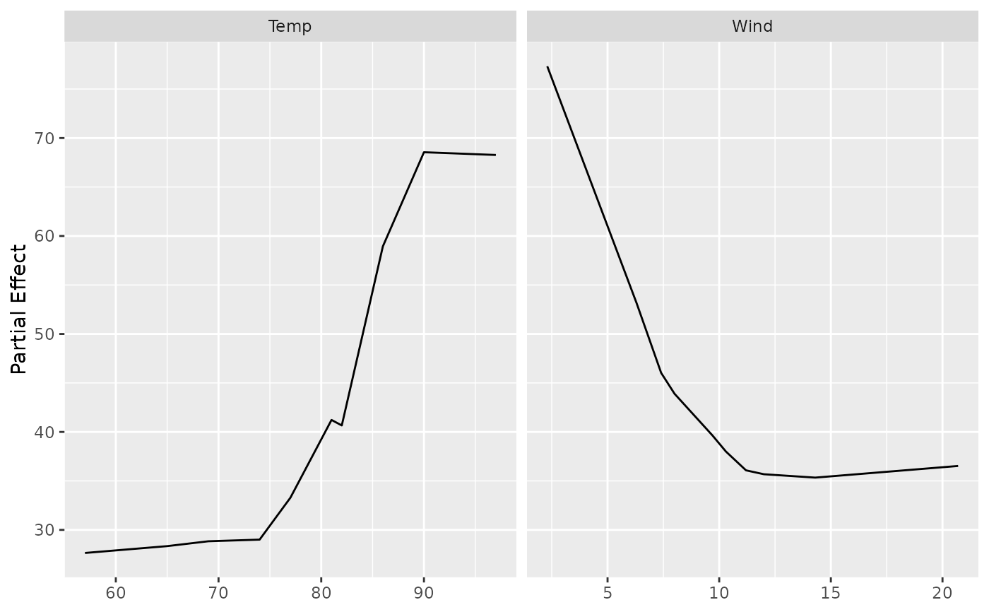
For a standard regression or classification forest, continuous predictors are drawn as line plots and categorical predictors as box plots, both faceted by variable name, the same arrangement as plot.gg_partial. The categorical data hold one prediction per training observation per level, not their average, so each box shows the spread of the prediction at that level and its middle line the median. For a survival forest the boxes are filled by time horizon, and with xvar2.name by the level of the second variable. When a survival forest has both, the fill is the time horizon and each level of the second variable gets its own panel.

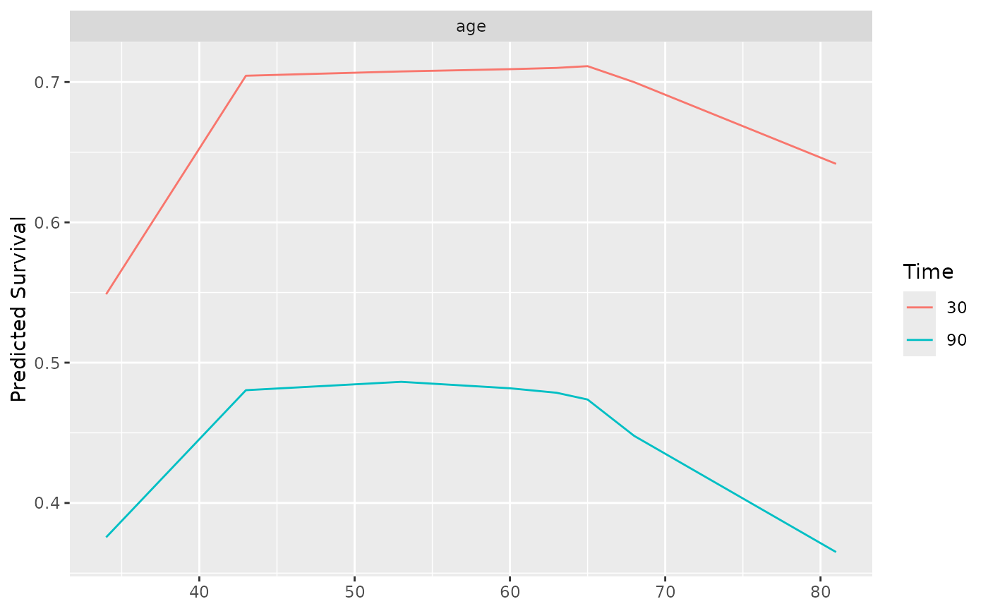
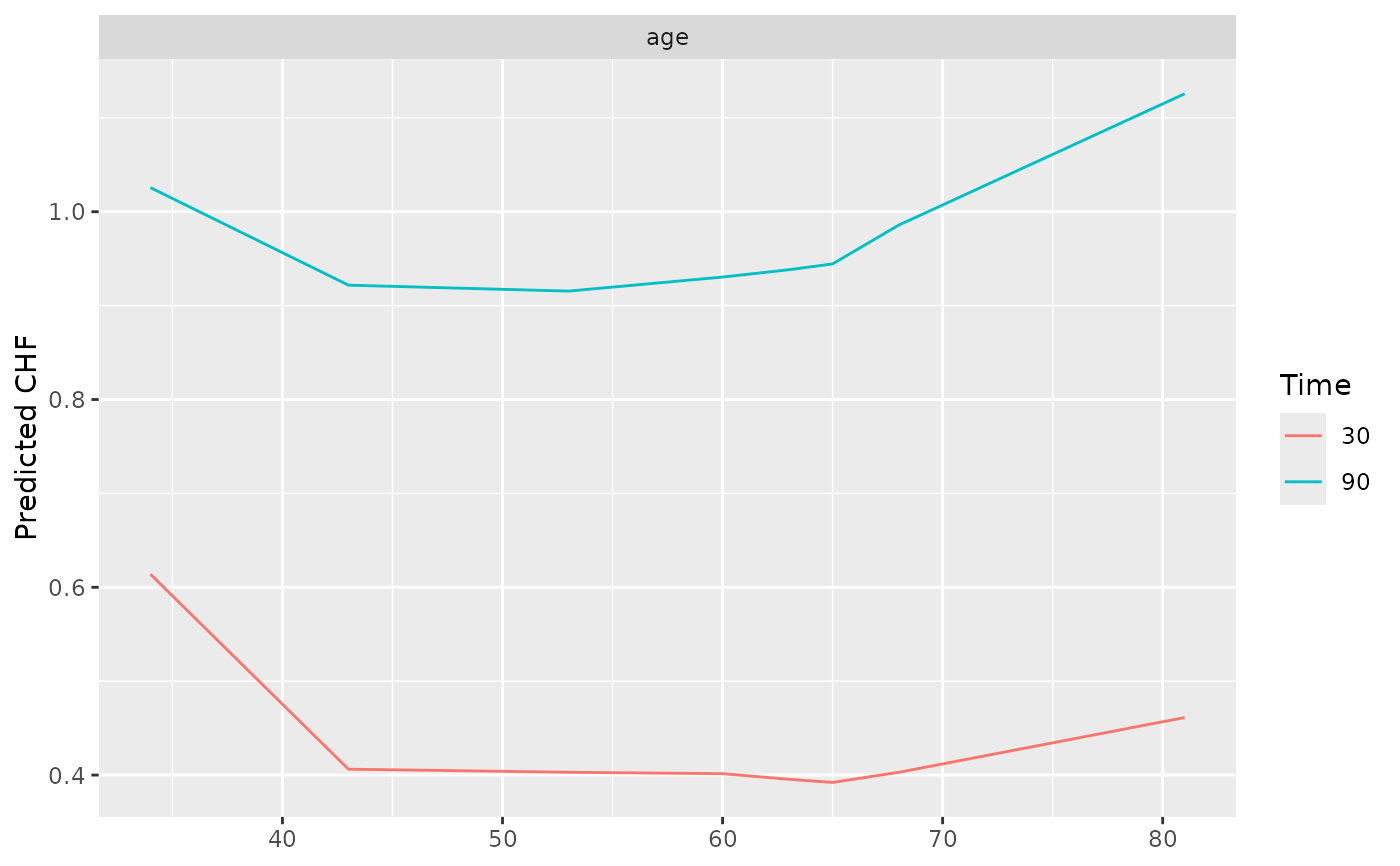
For a survival forest, each call to partial.rfsrc returns a predicted quantity (survival probability, cumulative hazard function, or mortality) at one or more chosen time horizons. When a time column is present in the data, each horizon becomes a separate colored curve over the predictor's value, still faceted by variable. Mortality has no time horizon, so it is drawn as a single curve. The y-axis label (“Predicted Survival”, “Predicted CHF”, or “Predicted Mortality”) tracks the partial.type attribute set by gg_partial_rfsrc().

For a two-variable interaction surface (when xvar2.name was supplied to gg_partial_rfsrc), the secondary variable's levels become separate colored lines, faceted by the primary predictor. On a survival forest the color is already the time horizon, so each level of the secondary variable gets its own panel instead, as in the categorical panel.

See also

gg_partial_rfsrc, plot.gg_partial

Examples

## ------------------------------------------------------------
## Regression forest -- one continuous curve per variable
## ------------------------------------------------------------
set.seed(42)
airq <- na.omit(airquality)
rfsrc_airq <- randomForestSRC::rfsrc(Ozone ~ ., data = airq, ntree = 50)

pd <- gg_partial_rfsrc(rfsrc_airq, xvar.names = c("Wind", "Temp"),
                       n_eval = 10)
plot(pd)


# \donttest{
## ------------------------------------------------------------
## Survival forest -- one curve per requested time horizon,
## faceted by variable. Y-axis label tracks `partial.type`.
## ------------------------------------------------------------
# randomForestSRC's formula parser requires the unqualified Surv() symbol;
# it Depends on `survival`, so Surv is on the search path once
# randomForestSRC is loaded.
data(veteran, package = "randomForestSRC")
set.seed(42)
rfsrc_v <- randomForestSRC::rfsrc(Surv(time, status) ~ .,
                                  data = veteran, ntree = 50)
ti  <- rfsrc_v$time.interest
t30 <- ti[which.min(abs(ti - 30))]
t90 <- ti[which.min(abs(ti - 90))]

# Default partial.type = "surv" -> y-axis "Predicted Survival"
pd_s <- gg_partial_rfsrc(rfsrc_v, xvar.names = "age",
                         partial.time = c(t30, t90), n_eval = 8)
plot(pd_s)


# partial.type = "chf" -> y-axis "Predicted CHF"
pd_c <- gg_partial_rfsrc(rfsrc_v, xvar.names = "age",
                         partial.time = c(t30, t90),
                         partial.type = "chf", n_eval = 8)
plot(pd_c)

# }