Most survival data begin with one row per subject: a follow-up time, an event indicator, and covariates measured at baseline. That row cannot show a covariate changing during follow-up. A Random Hazard Forest (RHF) instead accepts repeated time intervals for each subject, so a tree can use the covariate values that belong to each part of the subject’s path (Ishwaran et al. 2026; Ishwaran and Kogalur 2026).
This vignette uses simulated counting-process data to show how ggRandomForests reads an RHF fit. We first make the time-dependent data structure explicit, then extract case-specific hazard and cumulative hazard curves. The fitting, performance, importance, and tuning work has already been run by vignettes/precompute_rhf.R. The article evaluates only the inexpensive ggRandomForests extraction and plotting steps.
What changes with counting-process data?
One subject can contribute several rows. Each row covers an interval , and event records whether the event occurs at that interval’s right endpoint. The first simulated subject makes the layout concrete:
rhf_data <- bundle$data
one_subject <- rhf_data[rhf_data$id == rhf_data$id[1L],
                        c("id", "start", "stop", "event", "xtd")]
knitr::kable(one_subject, digits = 3)
| 1 |
0.000 |
0.082 |
0 |
0.054 |
| 1 |
0.082 |
0.121 |
0 |
0.080 |
| 1 |
0.121 |
0.185 |
0 |
0.122 |
| 1 |
0.185 |
0.313 |
1 |
0.207 |
The intervals do more than divide follow-up into pieces. They define a covariate path. A time-dependent covariate must be predictable: the value used at time is known just before the event decision at . In the first RHF simulation, the actual identity is xtd = (x.4 + x.5) * stop. Because this is a continuous function of time and the subject’s fixed x.4 and x.5, its value at stop is also its left-hand limit there. It is available for the interval ending at that time.
In data collected in practice, a lab value measured after an interval ends cannot be copied backward into that interval. At any candidate split time, the subject must be routed using the active record, not a later measurement. This is the no-lookahead rule: future covariate values never select an earlier branch. The active-record stitching and tree routing are behavior of randomForestRHF::rhf(), not ggRandomForests. ggRandomForests reads the fitted estimates after the upstream model has applied those rules (Ishwaran et al. 2026; Ishwaran and Kogalur 2026).
Here is a compact view of the full simulated data set:
records_per_subject <- as.integer(table(rhf_data$id))
events_by_subject <- tapply(rhf_data$event, rhf_data$id, max)
data_summary <- data.frame(
  measure = c(
    "Subjects",
    "Counting-process records",
    "Records per subject",
    "Subjects with an event",
    "xtd range"
  ),
  value = c(
    length(unique(rhf_data$id)),
    nrow(rhf_data),
    sprintf(
      "%d to %d (median %g)",
      min(records_per_subject),
      max(records_per_subject),
      stats::median(records_per_subject)
    ),
    sum(events_by_subject),
    sprintf("%.3f to %.3f", min(rhf_data$xtd), max(rhf_data$xtd))
  )
)
knitr::kable(data_summary, col.names = c("Measure", "Value"))
| Subjects |
500 |
| Counting-process records |
2598 |
| Records per subject |
2 to 7 (median 5) |
| Subjects with an event |
427 |
| xtd range |
0.000 to 0.975 |
Where did the fitted objects come from?
The preparation below is shown but not evaluated while the vignette renders. These are the fixed calls used to create the saved bundle. Keeping the upstream objects in rhf_precomputed.rds makes CRAN builds predictable, while vignettes/precompute_rhf.R lets you reproduce the bundle from the same public simulation whenever you want to rerun the longer calculations.
set.seed(20260825L)
sim <- randomForestRHF::hazard.simulation(1)
data <- sim$dta
formula <- stats::as.formula("Surv(id, start, stop, event) ~ .")
with(data, stopifnot(identical(xtd, (x.4 + x.5) * stop)))

fit <- randomForestRHF::rhf(
  formula, data, ntree = 50L, seed = -1L
)
auct_cumulative <- randomForestRHF::auct.rhf(
  fit, marker = "cumhaz", method = "cumulative", verbose = FALSE
)
auct_incident <- randomForestRHF::auct.rhf(
  fit, marker = "hazard", method = "incident",
  riskset = "subject", verbose = FALSE
)
cache <- randomForestRHF::varpro.cache.rhf(
  fit, max.rules.tree = 30L, max.tree = 20L, verbose = FALSE
)
time_index <- unique(as.integer(round(seq.int(
  1L, cache$K, length.out = 5L
))))
importance <- randomForestRHF::importance.rhf(
  fit, cache = cache, time.index = time_index, verbose = FALSE
)
tune_risk <- randomForestRHF::tune.treesize.rhf(
  formula, data, ntree = 20L, perf = "risk", lower = 2L,
  upper = 6L, max.evals = 5L, seed = 20260825L, verbose = FALSE,
  forest = FALSE
)
tune_iauc <- randomForestRHF::tune.iAUC.rhf(
  formula, data, ntree = 20L, lower = 2L, upper = 6L,
  max.evals = 5L, seed = 20260825L, verbose = FALSE,
  forest = FALSE
)
The loaded fit can be checked without growing another forest:
fit_summary <- data.frame(
  measure = c(
    "Object class",
    "Trees",
    "Subjects",
    "Working time points",
    "Saved ensemble source"
  ),
  value = c(
    paste(class(bundle$fit), collapse = ", "),
    bundle$fit$ntree,
    length(bundle$fit$ensemble.id),
    length(bundle$fit$time.interest),
    "out-of-bag hazard and cumulative hazard"
  )
)
knitr::kable(fit_summary, col.names = c("Fit component", "Value"))
| Object class |
rhf, grow, surv-tdc |
| Trees |
50 |
| Subjects |
500 |
| Working time points |
42 |
| Saved ensemble source |
out-of-bag hazard and cumulative hazard |
How do hazard and cumulative hazard differ?
gg_rhf() extracts both estimates into one tidy object, with one row for each subject and point on the RHF working time grid. This extraction runs live when the article renders:
#>   id       time    hazard         chf source
#> 1  1 0.01055113 0.9265708 0.009776536    oob
#> 2  2 0.01055113 0.1961717 0.002069869    oob
#> 3  3 0.01055113 1.8109938 0.019108357    oob
#> 4  4 0.01055113 0.7639137 0.008060290    oob
#> 5  5 0.01055113 0.8986797 0.009482248    oob
#> 6  6 0.01055113 3.5193765 0.037134033    oob
The source column is "oob" here, so each displayed curve uses the trees for which that subject was out of bag. We select six subjects only to keep the lines readable; the extracted object contains all 500.
Hazard is local
case_ids <- c(1, 2, 3, 11, 14, 22)
plot(rhf_curves, idx = case_ids)
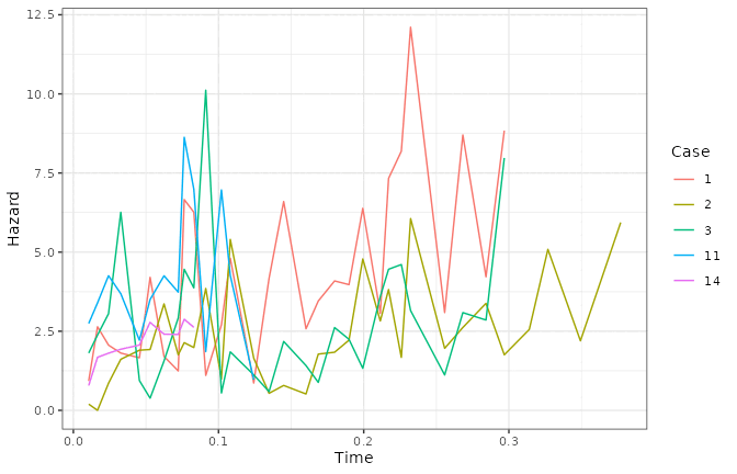
Hazard is a local event rate. A high point says that events are occurring at a high instantaneous rate among subjects still at risk around that time. It is not the probability that a subject has the event at that time, so neither its height nor its scale should be read as a percentage. RHF estimates this local quantity directly (Ishwaran et al. 2026).
Why do the hazard curves stop early?
Each line ends where that subject’s follow-up ends. This is upstream behavior: from version 2.0.0, randomForestRHF::rhf() returns a pointwise hazard only where a grid point falls inside one of the subject’s supplied (start, stop] records, and NA everywhere else, both in the gaps between records and after the final stop time. Earlier versions carried an estimate across the whole grid. gg_rhf() passes those NA values through unchanged, and plot() drops them before drawing, so a curve covers the range the forest was asked about and no more.
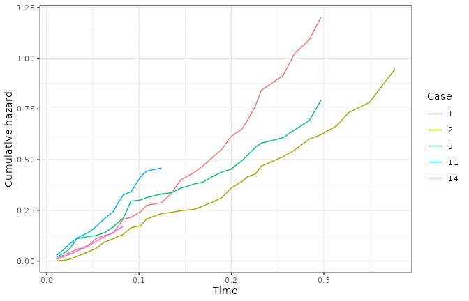
Cumulative hazard is masked too, but on a different rule, and version 2.0.3 changed it. It accumulates the exact overlap between the working grid and the supplied records, so it stays flat through a gap between two records rather than going missing there. After a subject’s final stop, though, there is no more overlap to accumulate, and from 2.0.3 the value is NA instead of the last level carried forward. So the cumulative-hazard panel below ends each curve where the hazard panel does, and the difference between the two masks only shows up on a fit with time-dependent covariates, where the gaps are real. If you summarize either column yourself, remember to pass na.rm = TRUE.
Cumulative hazard adds the local rates
The same gg_rhf object carries chf. Set the public hazard.only argument to FALSE to draw it:
plot(rhf_curves, idx = case_ids, hazard.only = FALSE)
The cumulative hazard function (CHF) adds hazard over follow-up. It summarizes accumulated event pressure, but it is unbounded and is not an event probability. Its scale answers “how much hazard has accumulated?”, while the hazard plot answers “where is the event rate high right now?”
There is one wrinkle in these time-dependent curves. randomForestRHF stitches record-specific ensemble estimates as each subject’s active record changes. A new record’s estimated CHF can start below the preceding record’s value, so a stitched case curve may contain a downward step. That step does not mean a negative hazard or that past event pressure disappeared. It marks the upstream model’s transition to a different active-record estimate (Ishwaran and Kogalur 2026).
How does discrimination change over time?
Survival AUC needs a definition of a case and a control at each time. The two definitions below answer different questions, and each uses the marker that matches its question. The saved AUC calculations are supplied to gg_auct(); only the extraction and plotting run during this render. Each call below still names its own method, which the saved fit already fixes, so that dropping auct_fit and letting gg_auct() compute leaves the chunk asking for the same estimand instead of falling back to the "cumulative" default.
Cumulative/dynamic AUC uses cumulative hazard
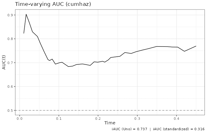
Suppose the question is whether a subject who has experienced the event by a horizon ranks above a subject who remains event-free at that horizon. This is the cumulative/dynamic target. The corresponding marker is cumulative hazard, named "chf" in gg_auct() and "cumhaz" in the retained upstream object.
auct_cumulative <- gg_auct(
  bundle$fit,
  marker = "chf",
  method = "cumulative",
  auct_fit = bundle$auct_cumulative
)
plot(auct_cumulative)
The saved curve has a Uno iAUC of 0.737. Its finite AUC values range from 0.684 to 0.903 over this fitted time grid. AUC is a ranking probability on a 0 to 1 scale, with 0.5 shown as the chance reference. The retained calculation did not use a bootstrap, so the plot has no confidence ribbon.
This curve needs randomForestRHF 2.0.3 or newer, which is why the package asks for that version. Before 2.0.3, auct.rhf() could put the cumulative/dynamic curve below the chance line on data the forest fits well. That was upstream rather than in gg_auct(), which passes the values through unchanged either way.
Incident/dynamic AUC uses hazard
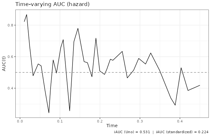
A different question asks whether a subject who experiences the event near time ranks above a subject in the relevant risk set at . This is the incident/dynamic target. It uses the local hazard marker, named "haz" in gg_auct() and "hazard" upstream.
auct_incident <- gg_auct(
  bundle$fit,
  marker = "haz",
  method = "incident",
  riskset = "subject",
  auct_fit = bundle$auct_incident
)
plot(auct_incident)
Here the Uno iAUC is 0.531. The curve is more variable than the cumulative/dynamic curve, with finite AUC values from 0.244 to 0.867. These values do not show that one marker is a better version of the other. Cumulative/dynamic AUC ranks accumulated risk through a horizon, while incident/dynamic AUC ranks local failures within a risk set. They estimate different targets.
Which variables matter, and when?
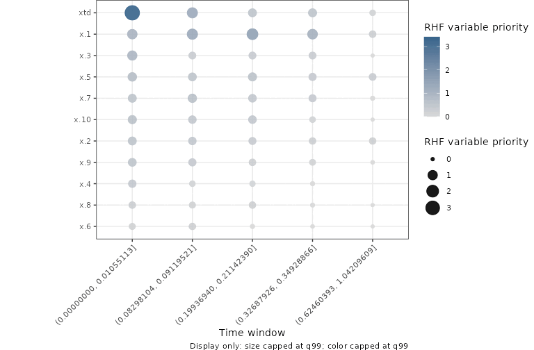
The retained importance.rhf object is the starting point here. Its expensive upstream work was performed once: varpro.cache.rhf() collected the rule and near-miss information, then importance.rhf() evaluated five selected time windows. Supplying that result avoids repeating either calculation.
RHF priority is a time-local rule-release contrast. Within a window, it compares the log integrated-hazard working response for a rule with its near-miss set and asks how much that fitted response changes when rules involving a variable are released. Larger nonnegative values in this supplied object mean a larger contrast. They do not say that a covariate raises or lowers hazard, and they are not z-scores, p-values, or automatic variable selection thresholds.
The dot size and color show the same priority value, with a 99th-percentile cap applied to the display only. The extracted values do not change. In this simulation, xtd has the largest early-window value, about 5.51, while x.1 has the largest value in several later windows. The number at risk falls from 779 to 32 across the five displayed windows, so the late-window comparisons use less information. One late x.4 result is unavailable in the upstream object and appears without a point. For work you plan to revisit, retain both the upstream cache and the importance.rhf result; supply the latter to gg_rhf_importance() for each display.
Which tree size did the upstream searches select?
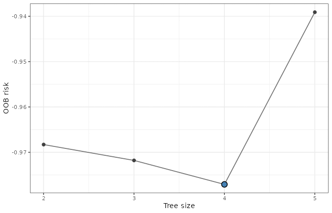
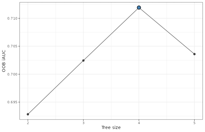
The two retained tune.treesize.rhf objects contain the evaluated paths and their selected sizes. gg_tune_rhf() preserves the upstream evaluation order, so the connecting line follows the order in which candidates were evaluated, not a newly sorted sequence. The emphasized point marks the size selected by the upstream search.
OOB risk tuning
risk_tuning <- gg_tune_rhf(bundle$tune_risk)
risk_tuning
#> <gg_tune_rhf> n: 4 | metric: OOB risk evaluations: 4 | selected treesize: 4 value: -0.9771
The risk search evaluated tree sizes 2, 3, 4, 5 in that order and selected size 4, where the saved mean OOB risk was smallest. The retained risk path has no standard-error field. gg_tune_rhf() sets its se values to missing and does not fabricate uncertainty, so a risk plot has no ribbon.
OOB iAUC tuning
iauc_tuning <- gg_tune_rhf(bundle$tune_iauc)
iauc_tuning
#> <gg_tune_rhf> n: 4 | metric: OOB iAUC evaluations: 4 | selected treesize: 4 value: 0.7119
The iAUC search evaluated tree sizes 2, 3, 4, 5 and selected size 4, where OOB iAUC was largest. An iAUC ribbon is drawn only when finite upstream standard errors are present. This saved path has 0 finite standard errors, so its plot has no ribbon. Retaining each tuning result preserves the actual candidate path, search order, and selected point without rerunning the fits.
All four families keep extraction separate from plotting. The intermediate object is a data frame with an added class, so you can inspect it before calling plot().
support <- data.frame(
  extractor = c(
    "gg_rhf()",
    "gg_auct()",
    "gg_rhf_importance()",
    "gg_tune_rhf()"
  ),
  upstream_input = c(
    "rhf fit",
    "rhf fit plus an optional auct.rhf object",
    "rhf fit plus an optional importance.rhf object",
    "tune.treesize.rhf object"
  ),
  returned_class = c(
    "gg_rhf, data.frame",
    "gg_auct, data.frame",
    "gg_rhf_importance, data.frame",
    "gg_tune_rhf, data.frame"
  ),
  scale = c(
    paste(
      "Hazard is a local event rate; cumulative hazard is accumulated",
      "event pressure. Neither is a probability."
    ),
    paste(
      "AUC(t) and iAUC are ranking measures from 0 to 1; interpretation",
      "depends on the case definition and marker."
    ),
    paste(
      "Time-local rule-release priority; larger values mean a larger",
      "working-response contrast, not statistical significance."
    ),
    paste(
      "OOB risk is minimized or OOB iAUC is maximized; the selected",
      "tree size is marked."
    )
  ),
  check.names = FALSE
)
knitr::kable(
  support,
  col.names = c(
    "Extractor", "Upstream input class or object",
    "Returned class", "Output scale and interpretation"
  )
)
| gg_rhf() |
rhf fit |
gg_rhf, data.frame |
Hazard is a local event rate; cumulative hazard is accumulated event pressure. Neither is a probability. |
| gg_auct() |
rhf fit plus an optional auct.rhf object |
gg_auct, data.frame |
AUC(t) and iAUC are ranking measures from 0 to 1; interpretation depends on the case definition and marker. |
| gg_rhf_importance() |
rhf fit plus an optional importance.rhf object |
gg_rhf_importance, data.frame |
Time-local rule-release priority; larger values mean a larger working-response contrast, not statistical significance. |
| gg_tune_rhf() |
tune.treesize.rhf object |
gg_tune_rhf, data.frame |
OOB risk is minimized or OOB iAUC is maximized; the selected tree size is marked. |
How can this analysis be reproduced?
The bundle records the public simulation, seed, calculation settings, and package versions used for this render. These are the saved versions:
version_table <- data.frame(
  package = names(bundle$versions),
  version = unname(bundle$versions),
  row.names = NULL
)
knitr::kable(
  version_table,
  col.names = c("Software", "Saved version")
)
| R |
4.6.1 |
| ggRandomForests |
4.0.0 |
| randomForestRHF |
2.0.3 |
| ggplot2 |
4.0.3 |
Run Rscript vignettes/precompute_rhf.R from the package root to regenerate all ten bundle components. That script repeats the sole longitudinal simulation and uses bundle$seed and the settings shown earlier. The exact numerical result can still change when the recorded package versions change.
For routine use, retain the fitted forest and each expensive upstream result: the two auct.rhf calculations, the importance cache and result, and both tuning objects. Supplying those objects is the default workflow for a report you expect to render more than once. It separates a long model calculation from a short, repeatable extraction and plot.
Further reading
The RHF method, including its counting-process construction and hazard-based forest, is described by Ishwaran, Hsich, Kogalur, and Lee (Ishwaran et al. 2026). The randomForestRHF software reference documents the R implementation and the upstream objects used throughout this article (Ishwaran and Kogalur 2026).
Ishwaran, Hemant, Eileen M. Hsich, Udaya B. Kogalur, and Donald K. K. Lee. 2026.
“Random Hazard Forests.” arXiv Preprint, ahead of print.
https://doi.org/10.48550/arXiv.2608.21597.
Ishwaran, Hemant, and Udaya B. Kogalur. 2026.
randomForestRHF: Random Hazard Forests.
https://CRAN.R-project.org/package=randomForestRHF.