Creates a hazard object and optionally fits it via maximum likelihood.
This mirrors the argument-oriented workflow of the legacy HAZARD C/SAS
implementation: supply starting values in theta and the function will
optimize to produce fitted estimates.
Usage
hazard(
  formula = NULL,
  data = NULL,
  time = NULL,
  status = NULL,
  time_lower = NULL,
  time_upper = NULL,
  x = NULL,
  time_windows = NULL,
  theta = NULL,
  dist = "weibull",
  phases = NULL,
  fit = FALSE,
  weights = NULL,
  control = list(),
  ...
)
Arguments
- formula
Optional formula of the form
Surv(time, status) ~ predictors. When provided, overrides direct time/status/x arguments and extracts from data. Example:hazard(Surv(time, status) ~ x1 + x2, data = df, dist = "weibull", fit = TRUE).- data
Optional data frame containing variables referenced in formula.
- time
Numeric follow-up time vector.
- status
Numeric or logical event indicator vector.
- time_lower
Optional numeric lower bound vector for censoring intervals. Used when
status == 2(interval-censored); defaults totimeif NULL.- time_upper
Optional numeric upper bound vector for censoring intervals. Used when
status %in% c(-1, 2); defaults totimeif NULL.- x
Optional design matrix (or data frame coercible to matrix).
- time_windows
Optional numeric vector of strictly positive cut points for piecewise time-varying coefficients. When provided, each predictor column in
xis expanded into one column per time window so each window gets its own coefficient.- theta
Optional numeric coefficient vector (starting values for optimization).
- dist
Character baseline distribution label (default
"weibull"). One of"weibull","exponential","loglogistic","lognormal", or"multiphase". The single-distribution families differ in the shape the hazard traces over time;"multiphase"builds an additive N-phase hazard and requiresphases. See the Baseline distributions section for what each means and when to use it.- phases
Optional named list of
hzr_phase()objects specifying the phases for a multiphase model (dist = "multiphase"). See Examples.- fit
Logical; if TRUE, fit the model via maximum likelihood (default FALSE).
- weights
Optional numeric vector of observation weights (non-negative). Each observation's log-likelihood contribution is multiplied by its weight. Use for severity-weighted repeated events. Default
NULL(unit weights). Implements the SASWEIGHTstatement.- control
Named list of control options (see Details).
- ...
Additional named arguments retained for parity with legacy calling conventions.
Value
An object of class hazard, a named list with components:
call (the matched call),
spec (model specification: dist, control,
time_windows, phases),
data (input data: time, status, x,
weights, etc.),
fit (optimisation results: theta, objective,
converged, se, vcov, counts, message;
all NULL when fit = FALSE),
and engine (implementation tag, "native-r-m2").
Details
Control parameters:
maxit: Maximum iterations (default 1000)n_starts: Number of optimization starts for multiphase fits (default 5). Each start after the first adds random noise to the initial values, drawn from the ambient RNG stream; callset.seed()before fitting for reproducible results.reltol: Relative parameter change tolerance (default 1e-5)abstol: Absolute gradient norm tolerance (default 1e-6)method: Optimization method: "bfgs" or "nm" (default "bfgs")condition: Condition number control (default 14)nocov,nocor: Suppress covariance/correlation output (legacy; no-op in M2)
Censoring status coding:
1: Exact event at time
0: Right-censored at time
-1: Left-censored with upper bound at time_upper \(or time\)
2: Interval-censored in the interval \(time_lower, time_upper\)
Time-varying coefficients:
If
time_windowsis supplied, predictors are expanded to piecewise window interactions so each window has its own coefficient vector.This is implemented as design-matrix expansion, so the existing likelihood engines remain unchanged.
The fitted model
For dist = "multiphase" the cumulative hazard, instantaneous hazard, and
survival are
$$H(t \mid \mathbf{x}) = \sum_{j=1}^{J} \mu_j(\mathbf{x}) \, \Phi_j(t), \qquad h(t \mid \mathbf{x}) = \sum_{j=1}^{J} \mu_j(\mathbf{x}) \, \varphi_j(t), \qquad S(t \mid \mathbf{x}) = \exp\!\bigl(-H(t \mid \mathbf{x})\bigr)$$
where \(\mu_j(\mathbf{x}) = \exp(\alpha_j + \mathbf{x}_j^\top
\beta_j)\) and the temporal shapes \(\Phi_j\), \(\varphi_j\)
are set by each phase's type (see hzr_phase()). The
proportional-hazards single-phase families ("weibull", "exponential")
are the special case \(J = 1\), with covariates acting multiplicatively on
one temporal shape. The "loglogistic" (proportional-odds) and
"lognormal" (accelerated-failure-time) families place covariates
differently — on the odds of failure and the log-time location,
respectively — so they are separate parameterizations, not special cases
of this additive form. Parameters are estimated
on an unconstrained internal scale (e.g. \(\log\mu\), \(\log t_{1/2}\))
and transformed back for reporting; see
vignette("mf-mathematical-foundations").
Baseline distributions
The dist argument selects the parametric form of the baseline hazard. The
four single-distribution families differ in the shape the
hazard traces over follow-up; choose by what the risk is expected to do over
time. "multiphase" is the general additive model that lets several such
shapes coexist.
"weibull"— monotone rising or falling hazard (default)The workhorse parametric model: \(H(t \mid \mathbf{x}) = (\mu t)^\nu \exp(\eta)\), with hazard \(h \propto t^{\nu - 1}\). The single shape \(\nu\) makes risk increase over time (\(\nu > 1\)), decrease (\(\nu < 1\)), or stay flat (\(\nu = 1\)). Use it as the default when a single monotone trend describes the hazard.
"exponential"— constant hazardThe memoryless special case \(\nu = 1\): a time-invariant baseline rate, \(H(t \mid \mathbf{x}) = \mu t \exp(\eta)\). Use it when the event rate does not change with follow-up time (the constant background risk also appears as the
"constant"phase in a multiphase model)."loglogistic"— unimodal (rise-then-fall) hazardA log-logistic proportional-odds form (covariates act multiplicatively on the odds of failure, \(\exp(\eta)\), not as an AFT time shift) whose hazard rises to a single peak and then declines when the shape exceeds 1 (and is monotone decreasing otherwise), with heavier tails than the log-normal. Use it when risk climbs to an early peak and then eases off.
"lognormal"— early-peaking, resolving hazardAn accelerated-failure-time form in which \(\log\) time is Gaussian; the hazard rises to an early peak and then decays toward zero. Use it for risk that is concentrated early and resolves over time.
"multiphase"— additive N-phase hazardSums several phase shapes into one model, \(H = \sum_j \mu_j(\mathbf{x}) \Phi_j(t)\), so the overall hazard can fall, level off, and rise again within one fit. Requires
phases; seehzr_phase()for the available phase shapes. This is the form that reproduces the classic C/SAS HAZARD models.
References
Blackstone EH, Naftel DC, Turner ME Jr. The decomposition of time-varying hazard into phases, each incorporating a separate stream of concomitant information. J Am Stat Assoc. 1986;81(395):615–624. doi:10.1080/01621459.1986.10478314
Rajeswaran J, Blackstone EH, Ehrlinger J, Li L, Ishwaran H, Parides MK. Probability of atrial fibrillation after ablation: Using a parametric nonlinear temporal decomposition mixed effects model. Stat Methods Med Res. 2018;27(1):126–141. doi:10.1177/0962280215623583
See also
predict.hazard() for survival/cumulative-hazard predictions,
summary.hazard() for model summaries,
hzr_phase() for specifying multiphase temporal shapes.
Vignettes with worked examples:
vignette("fitting-hazard-models") — single-phase through multiphase fitting,
vignette("prediction-visualization") — prediction types and decomposed hazard plots,
vignette("inference-diagnostics") — bootstrap CIs and model diagnostics.
Examples
# -- Univariable Weibull ----------------------------------------------
set.seed(1)
time <- rexp(50, rate = 0.3)
status <- sample(0:1, 50, replace = TRUE, prob = c(0.3, 0.7))
fit <- hazard(time = time, status = status,
theta = c(0.3, 1.0), dist = "weibull", fit = TRUE)
summary(fit)
#> hazard model summary
#> observations: 50
#> predictors: 0
#> dist: weibull
#> engine: native-r-m2
#> converged: TRUE
#> log-lik: -89.5173
#> evaluations: fn=23, gr=7
#>
#> Coefficients:
#> estimate std_error z_stat p_value
#> mu 0.2190092 0.02728228 8.027524 9.945983e-16
#> nu 1.3389540 0.15829050 8.458840 2.700510e-17
# -- Formula interface with covariates --------------------------------
set.seed(1001)
n <- 180
dat <- data.frame(
time = rexp(n, rate = 0.35) + 0.05,
status = rbinom(n, size = 1, prob = 0.6),
age = rnorm(n, mean = 62, sd = 11),
nyha = sample(1:4, n, replace = TRUE),
shock = rbinom(n, size = 1, prob = 0.18)
)
fit2 <- hazard(
survival::Surv(time, status) ~ age + nyha + shock,
data = dat,
theta = c(mu = 0.25, nu = 1.10, beta1 = 0, beta2 = 0, beta3 = 0),
dist = "weibull",
fit = TRUE,
control = list(maxit = 300)
)
summary(fit2)
#> hazard model summary
#> observations: 180
#> predictors: 3
#> dist: weibull
#> engine: native-r-m2
#> converged: TRUE
#> log-lik: -293.553
#> evaluations: fn=36, gr=8
#>
#> Coefficients:
#> estimate std_error z_stat p_value
#> mu 0.121860518 0.062260593 1.95726560 5.031625e-02
#> nu 1.143730632 0.084302528 13.56697905 6.285984e-42
#> beta1 0.001716551 0.008807986 0.19488579 8.454824e-01
#> beta2 0.156208724 0.090597558 1.72420458 8.467092e-02
#> beta3 0.017352702 0.362918430 0.04781433 9.618642e-01
# \donttest{
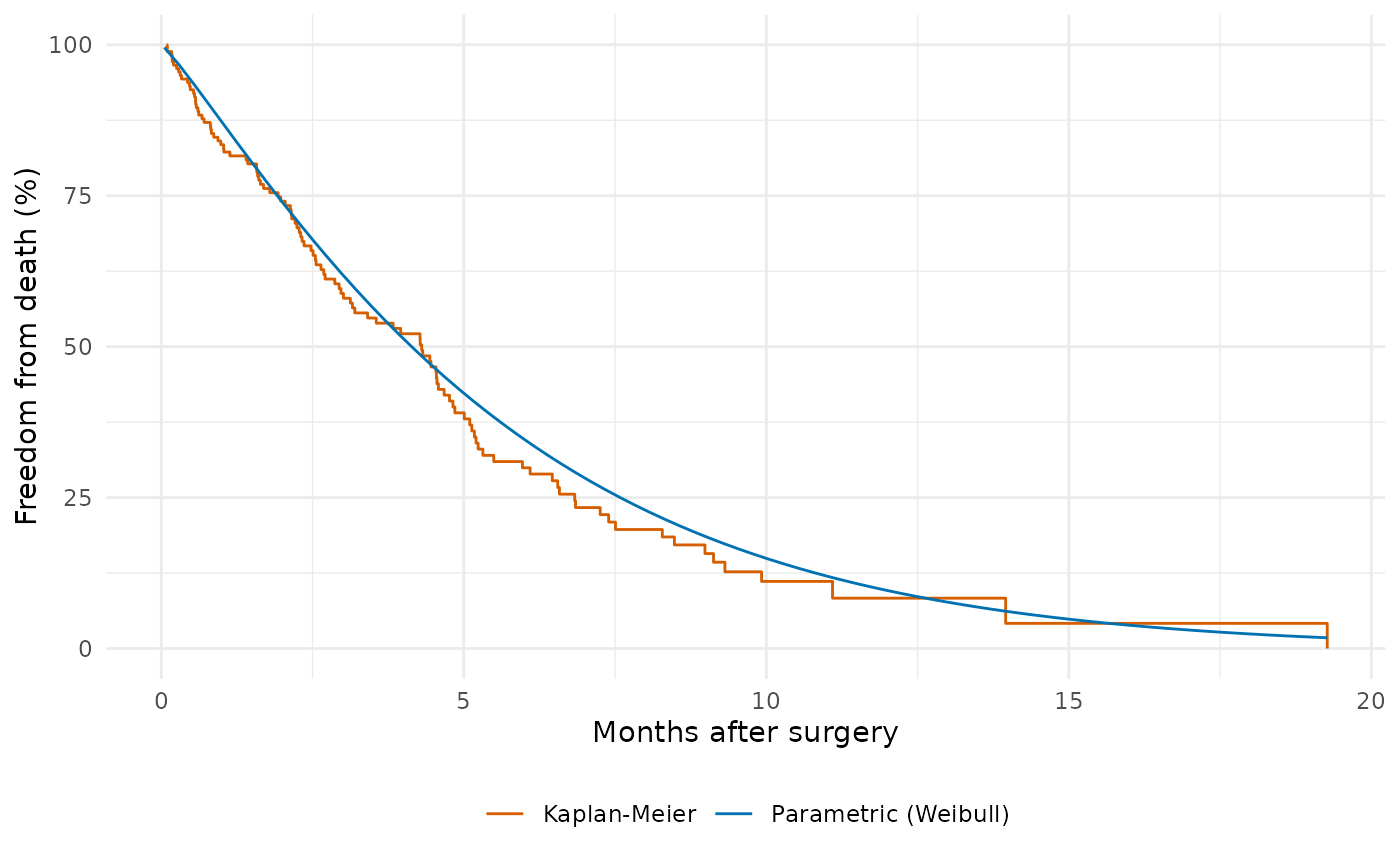
# -- Parametric survival with Kaplan-Meier overlay -----------------
if (requireNamespace("ggplot2", quietly = TRUE)) {
library(ggplot2)
# Parametric curve on a fine grid at median covariate profile
t_grid <- seq(0.05, max(dat$time), length.out = 80)
curve_df <- data.frame(
time = t_grid, age = median(dat$age), nyha = 2, shock = 0
)
curve_df$survival <- predict(fit2, newdata = curve_df,
type = "survival") * 100
# Kaplan-Meier empirical overlay
km <- survival::survfit(survival::Surv(time, status) ~ 1, data = dat)
km_df <- data.frame(time = km$time, survival = km$surv * 100)
ggplot() +
geom_step(data = km_df, aes(time, survival, colour = "Kaplan-Meier")) +
geom_line(data = curve_df, aes(time, survival,
colour = "Parametric (Weibull)")) +
scale_colour_manual(
values = c("Parametric (Weibull)" = "#0072B2",
"Kaplan-Meier" = "#D55E00")
) +
scale_y_continuous(limits = c(0, 100)) +
labs(x = "Months after surgery", y = "Freedom from death (%)",
colour = NULL) +
theme_minimal() +
theme(legend.position = "bottom")
}
 # }
# \donttest{
# -- Multiphase model (two phases) ---------------------------------
fit_mp <- hazard(
survival::Surv(time, status) ~ 1,
data = dat,
dist = "multiphase",
phases = list(
early = hzr_phase("cdf", t_half = 0.5, nu = 2, m = 0,
fixed = "shapes"),
late = hzr_phase("cdf", t_half = 5, nu = 1, m = 0,
fixed = "shapes")
),
fit = TRUE,
control = list(n_starts = 5, maxit = 1000)
)
#> Warning: hessian_fn returned a non-conformant result; using numerical Hessian
#> Warning: hessian_fn returned a non-conformant result; using numerical Hessian
#> Warning: hessian_fn returned a non-conformant result; using numerical Hessian
#> Warning: hessian_fn returned a non-conformant result; using numerical Hessian
#> Warning: hessian_fn returned a non-conformant result; using numerical Hessian
summary(fit_mp)
#> Multiphase hazard model (2 phases)
#> observations: 180
#> predictors: 0
#> dist: multiphase
#> phase 1: early - cdf (early risk)
#> phase 2: late - cdf (late risk)
#> engine: native-r-m2
#> converged: TRUE
#> log-lik: -321.926
#> evaluations: fn=16, gr=7
#>
#> Coefficients (internal scale):
#>
#> Phase: early (cdf)
#> estimate std_error z_stat p_value
#> log_mu -1.8209827 0.2701943 -6.739531 1.588985e-11
#> log_t_half -0.6931472 NA NA NA
#> nu 2.0000000 NA NA NA
#> m 0.0000000 NA NA NA
#>
#> Phase: late (cdf)
#> estimate std_error z_stat p_value
#> log_mu 0.6119202 0.1098498 5.570517 2.539839e-08
#> log_t_half 1.6094379 NA NA NA
#> nu 1.0000000 NA NA NA
#> m 0.0000000 NA NA NA
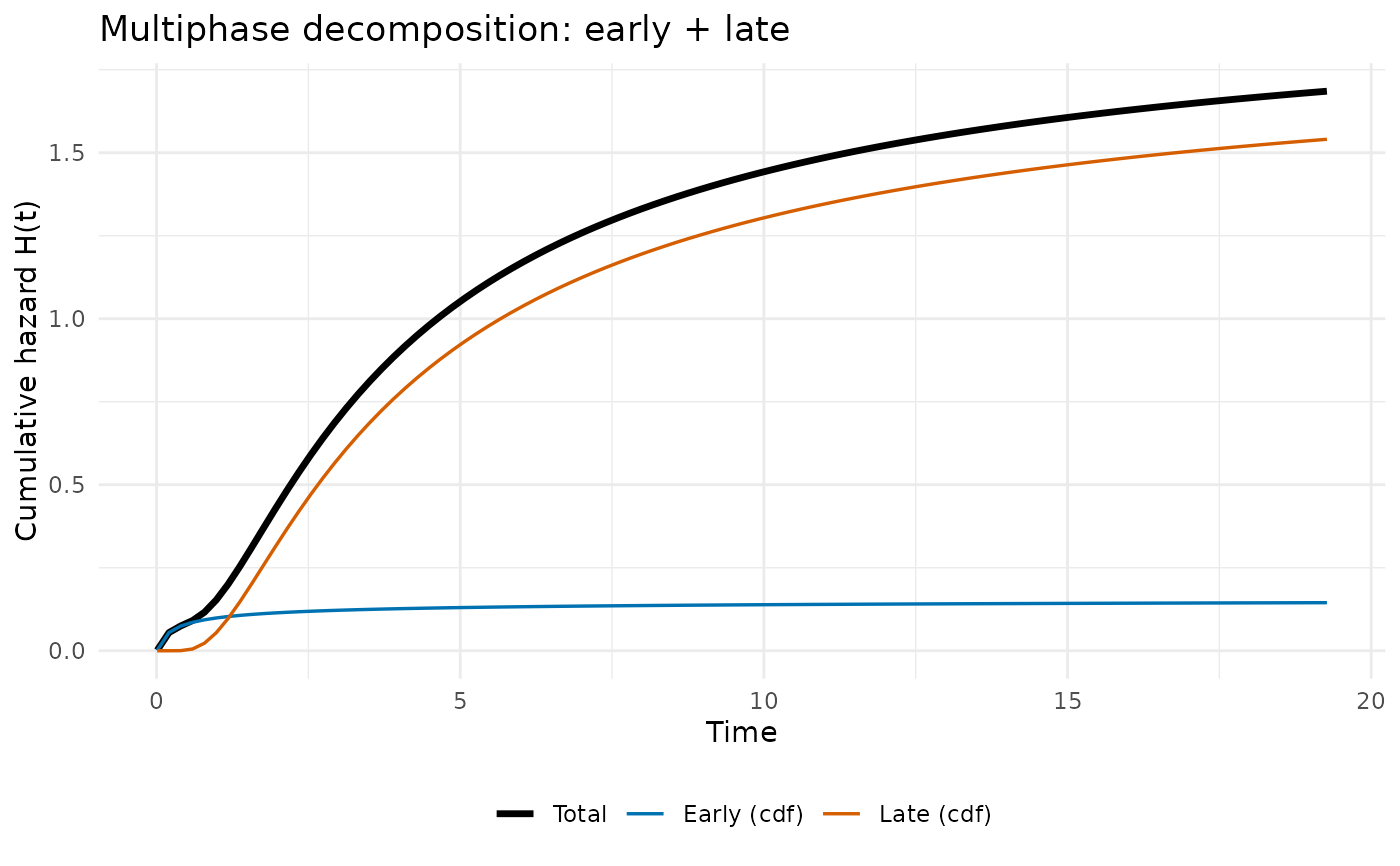
# -- Per-phase decomposed cumulative hazard ------------------------
if (requireNamespace("ggplot2", quietly = TRUE)) {
t_grid <- seq(0.01, max(dat$time), length.out = 100)
decomp <- predict(fit_mp, newdata = data.frame(time = t_grid),
type = "cumulative_hazard", decompose = TRUE)
df_long <- data.frame(
time = rep(decomp$time, 3),
cumhaz = c(decomp$total, decomp$early, decomp$late),
component = rep(c("Total", "Early (cdf)", "Late (cdf)"),
each = nrow(decomp))
)
df_long$component <- factor(df_long$component,
levels = c("Total", "Early (cdf)", "Late (cdf)"))
ggplot2::ggplot(df_long,
ggplot2::aes(x = time, y = cumhaz, colour = component,
linewidth = component)) +
ggplot2::geom_line() +
ggplot2::scale_colour_manual(values = c(
"Total" = "black", "Early (cdf)" = "#0072B2",
"Late (cdf)" = "#D55E00"
)) +
ggplot2::scale_linewidth_manual(values = c(
"Total" = 1.2, "Early (cdf)" = 0.6, "Late (cdf)" = 0.6
)) +
ggplot2::labs(
x = "Time", y = "Cumulative hazard H(t)",
colour = NULL, linewidth = NULL,
title = "Multiphase decomposition: early + late"
) +
ggplot2::theme_minimal() +
ggplot2::theme(legend.position = "bottom")
}
# }
# \donttest{
# -- Multiphase model (two phases) ---------------------------------
fit_mp <- hazard(
survival::Surv(time, status) ~ 1,
data = dat,
dist = "multiphase",
phases = list(
early = hzr_phase("cdf", t_half = 0.5, nu = 2, m = 0,
fixed = "shapes"),
late = hzr_phase("cdf", t_half = 5, nu = 1, m = 0,
fixed = "shapes")
),
fit = TRUE,
control = list(n_starts = 5, maxit = 1000)
)
#> Warning: hessian_fn returned a non-conformant result; using numerical Hessian
#> Warning: hessian_fn returned a non-conformant result; using numerical Hessian
#> Warning: hessian_fn returned a non-conformant result; using numerical Hessian
#> Warning: hessian_fn returned a non-conformant result; using numerical Hessian
#> Warning: hessian_fn returned a non-conformant result; using numerical Hessian
summary(fit_mp)
#> Multiphase hazard model (2 phases)
#> observations: 180
#> predictors: 0
#> dist: multiphase
#> phase 1: early - cdf (early risk)
#> phase 2: late - cdf (late risk)
#> engine: native-r-m2
#> converged: TRUE
#> log-lik: -321.926
#> evaluations: fn=16, gr=7
#>
#> Coefficients (internal scale):
#>
#> Phase: early (cdf)
#> estimate std_error z_stat p_value
#> log_mu -1.8209827 0.2701943 -6.739531 1.588985e-11
#> log_t_half -0.6931472 NA NA NA
#> nu 2.0000000 NA NA NA
#> m 0.0000000 NA NA NA
#>
#> Phase: late (cdf)
#> estimate std_error z_stat p_value
#> log_mu 0.6119202 0.1098498 5.570517 2.539839e-08
#> log_t_half 1.6094379 NA NA NA
#> nu 1.0000000 NA NA NA
#> m 0.0000000 NA NA NA
# -- Per-phase decomposed cumulative hazard ------------------------
if (requireNamespace("ggplot2", quietly = TRUE)) {
t_grid <- seq(0.01, max(dat$time), length.out = 100)
decomp <- predict(fit_mp, newdata = data.frame(time = t_grid),
type = "cumulative_hazard", decompose = TRUE)
df_long <- data.frame(
time = rep(decomp$time, 3),
cumhaz = c(decomp$total, decomp$early, decomp$late),
component = rep(c("Total", "Early (cdf)", "Late (cdf)"),
each = nrow(decomp))
)
df_long$component <- factor(df_long$component,
levels = c("Total", "Early (cdf)", "Late (cdf)"))
ggplot2::ggplot(df_long,
ggplot2::aes(x = time, y = cumhaz, colour = component,
linewidth = component)) +
ggplot2::geom_line() +
ggplot2::scale_colour_manual(values = c(
"Total" = "black", "Early (cdf)" = "#0072B2",
"Late (cdf)" = "#D55E00"
)) +
ggplot2::scale_linewidth_manual(values = c(
"Total" = 1.2, "Early (cdf)" = 0.6, "Late (cdf)" = 0.6
)) +
ggplot2::labs(
x = "Time", y = "Cumulative hazard H(t)",
colour = NULL, linewidth = NULL,
title = "Multiphase decomposition: early + late"
) +
ggplot2::theme_minimal() +
ggplot2::theme(legend.position = "bottom")
}
 # }
# }