Predict from a hazard model object

Produces prediction outputs from a hazard object. Supports multiple prediction types including linear predictor, hazard, survival probability, and cumulative hazard.

Usage

# S3 method for class 'hazard'
predict(
  object,
  newdata = NULL,
  type = c("hazard", "linear_predictor", "survival", "cumulative_hazard"),
  decompose = FALSE,
  ...
)

Arguments

object

A hazard object.

newdata

Optional matrix or data frame of predictors. For types requiring time (e.g., "survival", "cumulative_hazard"), newdata should include a time column, or time will be taken from the fitted object's data.

type

Prediction type:

"linear_predictor": Linear predictor eta = x*beta (not available for multiphase)
"hazard": Hazard scale exp(eta) (not available for multiphase)
"survival": Survival probability S(t|x) = exp(-H(t|x))
"cumulative_hazard": Cumulative hazard H(t|x) at event times

decompose

Logical; if TRUE and the model is multiphase, return a data frame with per-phase cumulative hazard contributions alongside the total. Ignored for single-distribution models. Default FALSE.

...

Unused; included for S3 compatibility.

Value

Numeric vector of predictions.

Details

For Weibull models with survival or cumulative_hazard predictions:

Cumulative hazard: H(t|x) = (mu*t)^nu * exp(eta)
Survival: S(t|x) = exp(-H(t|x))

Time values must be positive and finite. If newdata contains a time column, it will be used; otherwise, the time vector from the fitted object is used. For models fit with time_windows, predictions for type = "linear_predictor" or "hazard" also require time values (via newdata$time or fitted-time fallback) so window-specific coefficients can be selected.

Examples

# -- Basic predictions ------------------------------------------------
set.seed(1)
fit <- hazard(time = rexp(50, 0.3), status = rep(1L, 50),
              theta = c(0.3, 1.0), dist = "weibull", fit = TRUE)
predict(fit, type = "survival")
#>  [1] 0.508448836 0.315117497 0.909632142 0.913801355 0.704022509 0.034429522
#>  [7] 0.297904379 0.635876619 0.407732732 0.908685617 0.245861859 0.504733067
#> [13] 0.295096862 0.003729697 0.364948062 0.373066533 0.134498594 0.565324696
#> [19] 0.772692686 0.605268524 0.070992893 0.572924045 0.803140735 0.619329758
#> [25] 0.937239852 0.968075472 0.611315229 0.007471798 0.318195648 0.389681823
#> [31] 0.232969073 0.981596565 0.781843506 0.267479469 0.868327070 0.378412625
#> [37] 0.797695039 0.524953194 0.510431884 0.845615583 0.354514703 0.376046945
#> [43] 0.276615587 0.289749395 0.626388405 0.798022001 0.276332062 0.390676459
#> [49] 0.652266897 0.113525051
predict(fit, newdata = data.frame(time = c(1, 2, 5)),
        type = "cumulative_hazard")
#> [1] 0.2244716 0.5138491 1.5356737

# -- Patient-specific survival curves ---------------------------------
set.seed(1001)
n   <- 180
dat <- data.frame(
  time   = rexp(n, rate = 0.35) + 0.05,
  status = rbinom(n, size = 1, prob = 0.6),
  age    = rnorm(n, mean = 62, sd = 11),
  nyha   = sample(1:4, n, replace = TRUE),
  shock  = rbinom(n, size = 1, prob = 0.18)
)
fit2 <- hazard(
  survival::Surv(time, status) ~ age + nyha + shock,
  data  = dat,
  theta = c(mu = 0.25, nu = 1.10, beta1 = 0, beta2 = 0, beta3 = 0),
  dist  = "weibull", fit = TRUE
)

new_patients <- data.frame(
  time = c(0.5, 1.5, 3.0),
  age  = c(50, 65, 75),
  nyha = c(1, 3, 4),
  shock = c(0, 0, 1)
)
# Compute predictions from the clean covariate frame before adding columns
surv   <- predict(fit2, newdata = new_patients, type = "survival")
cumhaz <- predict(fit2, newdata = new_patients, type = "cumulative_hazard")
new_patients$survival          <- surv
new_patients$cumulative_hazard <- cumhaz
new_patients
#>   time age nyha shock  survival cumulative_hazard
#> 1  0.5  50    1     0 0.9494097        0.05191482
#> 2  1.5  65    3     0 0.7743185        0.25577202
#> 3  3.0  75    4     1 0.5046535        0.68388317

# \donttest{
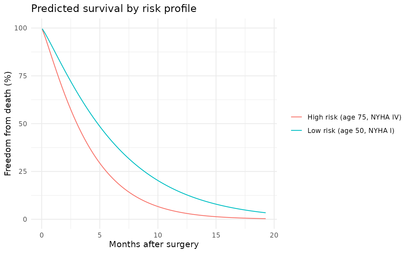
# -- Grouped survival curves ---------------------------------------
if (requireNamespace("ggplot2", quietly = TRUE)) {
  library(ggplot2)

  t_grid <- seq(0.05, max(dat$time), length.out = 80)
  profiles <- data.frame(
    label = c("Low risk (age 50, NYHA I)",
              "High risk (age 75, NYHA IV)"),
    age   = c(50, 75),
    nyha  = c(1, 4),
    shock = c(0, 1)
  )

  curve_list <- lapply(seq_len(nrow(profiles)), function(i) {
    nd <- data.frame(
      time  = t_grid,
      age   = profiles$age[i],
      nyha  = profiles$nyha[i],
      shock = profiles$shock[i]
    )
    nd$survival <- predict(fit2, newdata = nd, type = "survival") * 100
    nd$profile  <- profiles$label[i]
    nd
  })
  curve_df <- do.call(rbind, curve_list)

  ggplot(curve_df, aes(time, survival, colour = profile)) +
    geom_line() +
    scale_y_continuous(limits = c(0, 100)) +
    labs(x = "Months after surgery",
         y = "Freedom from death (%)",
         title = "Predicted survival by risk profile",
         colour = NULL) +
    theme_minimal()
}

# }

# \donttest{
# -- Multiphase predictions with decomposition --------------------
set.seed(42)
n   <- 200
dat <- data.frame(
  time   = rexp(n, rate = 0.25) + 0.01,
  status = rbinom(n, size = 1, prob = 0.65)
)
fit_mp <- hazard(
  survival::Surv(time, status) ~ 1,
  data   = dat,
  dist   = "multiphase",
  phases = list(
    early = hzr_phase("cdf", t_half = 0.5, nu = 2, m = 0,
                       fixed = "shapes"),
    late  = hzr_phase("cdf", t_half = 5,   nu = 1, m = 0,
                       fixed = "shapes")
  ),
  fit     = TRUE,
  control = list(n_starts = 5, maxit = 1000)
)

t_grid <- seq(0.01, max(dat$time) * 0.9, length.out = 100)
nd     <- data.frame(time = t_grid)

# Overall survival
predict(fit_mp, newdata = nd, type = "survival")
#> early.log_mu early.log_mu early.log_mu early.log_mu early.log_mu early.log_mu 
#>    0.9991035    0.9506793    0.9308162    0.8914472    0.8319967    0.7661083 
#> early.log_mu early.log_mu early.log_mu early.log_mu early.log_mu early.log_mu 
#>    0.7030012    0.6464729    0.5973334    0.5551219    0.5189604    0.4879204 
#> early.log_mu early.log_mu early.log_mu early.log_mu early.log_mu early.log_mu 
#>    0.4611599    0.4379618    0.4177323    0.3999852    0.3843243    0.3704264 
#> early.log_mu early.log_mu early.log_mu early.log_mu early.log_mu early.log_mu 
#>    0.3580275    0.3469102    0.3368953    0.3278339    0.3196015    0.3120937 
#> early.log_mu early.log_mu early.log_mu early.log_mu early.log_mu early.log_mu 
#>    0.3052222    0.2989121    0.2930993    0.2877292    0.2827542    0.2781335 
#> early.log_mu early.log_mu early.log_mu early.log_mu early.log_mu early.log_mu 
#>    0.2738314    0.2698169    0.2660626    0.2625446    0.2592417    0.2561351 
#> early.log_mu early.log_mu early.log_mu early.log_mu early.log_mu early.log_mu 
#>    0.2532082    0.2504459    0.2478352    0.2453639    0.2430214    0.2407981 
#> early.log_mu early.log_mu early.log_mu early.log_mu early.log_mu early.log_mu 
#>    0.2386851    0.2366746    0.2347594    0.2329329    0.2311892    0.2295228 
#> early.log_mu early.log_mu early.log_mu early.log_mu early.log_mu early.log_mu 
#>    0.2279288    0.2264026    0.2249400    0.2235372    0.2221905    0.2208967 
#> early.log_mu early.log_mu early.log_mu early.log_mu early.log_mu early.log_mu 
#>    0.2196529    0.2184561    0.2173037    0.2161934    0.2151230    0.2140902 
#> early.log_mu early.log_mu early.log_mu early.log_mu early.log_mu early.log_mu 
#>    0.2130932    0.2121302    0.2111994    0.2102993    0.2094284    0.2085853 
#> early.log_mu early.log_mu early.log_mu early.log_mu early.log_mu early.log_mu 
#>    0.2077688    0.2069774    0.2062103    0.2054661    0.2047440    0.2040429 
#> early.log_mu early.log_mu early.log_mu early.log_mu early.log_mu early.log_mu 
#>    0.2033620    0.2027005    0.2020574    0.2014320    0.2008237    0.2002317 
#> early.log_mu early.log_mu early.log_mu early.log_mu early.log_mu early.log_mu 
#>    0.1996554    0.1990942    0.1985474    0.1980146    0.1974952    0.1969888 
#> early.log_mu early.log_mu early.log_mu early.log_mu early.log_mu early.log_mu 
#>    0.1964947    0.1960127    0.1955422    0.1950828    0.1946343    0.1941961 
#> early.log_mu early.log_mu early.log_mu early.log_mu early.log_mu early.log_mu 
#>    0.1937679    0.1933494    0.1929403    0.1925402    0.1921489    0.1917661 
#> early.log_mu early.log_mu early.log_mu early.log_mu 
#>    0.1913914    0.1910247    0.1906657    0.1903142 

# Per-phase decomposed cumulative hazard
decomp <- predict(fit_mp, newdata = nd,
                  type = "cumulative_hazard", decompose = TRUE)
head(decomp)
#>        time        total        early          late
#> 1 0.0100000 0.0008968715 0.0008968715 5.301145e-151
#> 2 0.3177112 0.0505785158 0.0505467552  3.176063e-05
#> 3 0.6254224 0.0716934643 0.0648896246  6.803840e-03
#> 4 0.9331336 0.1149091204 0.0726070448  4.230208e-02
#> 5 1.2408448 0.1839268533 0.0776684396  1.062584e-01
#> 6 1.5485560 0.2664317832 0.0813355656  1.850962e-01
# }

Usage

Arguments

Value

Details

See also

Examples