Superseded.
survival_difference_plot() has been superseded by the S3 constructor
hv_survival_difference() plus plot.hv_survival_difference().
Pass a diffout dataset and you get the S_2(t) - S_1(t) curve with an
optional confidence band. Covers tp.hp.dead.life-gained.sas and the
survival-difference component of tp.hp.numtreat.survdiff.matched.sas.
SAS context: The HAZDIFL macro in tp.hp.dead.life-gained.sas
bootstraps the difference S_2(t) - S_1(t) (or S_1(t) - S_2(t)) and
stores the result in a diffout dataset. Export that dataset and pass it
here with the appropriate column names.
Usage
survival_difference_plot(
  diff_data,
  x_col = "time",
  estimate_col = "difference",
  lower_col = NULL,
  upper_col = NULL,
  group_col = NULL,
  ci_alpha = 0.2,
  line_width = 1
)
Arguments
- diff_data
Data frame of pre-computed survival differences. See
sample_survival_difference_data().- x_col
Name of the time column. Default
"time".- estimate_col
Name of the difference column. Default
"difference".- lower_col
Name of the lower CI column, or
NULL. DefaultNULL.- upper_col
Name of the upper CI column, or
NULL. DefaultNULL.- group_col
Name of a grouping column for multiple comparisons, or
NULL. DefaultNULL.- ci_alpha
Transparency of the CI ribbon. Default
0.20.- line_width
Line width. Default
1.0.
Value
A ggplot2::ggplot() object.
Examples
library(ggplot2)
diff_dat <- sample_survival_difference_data(
n = 500, time_max = 10,
groups = c("Control" = 1.0, "Treatment" = 0.70)
)
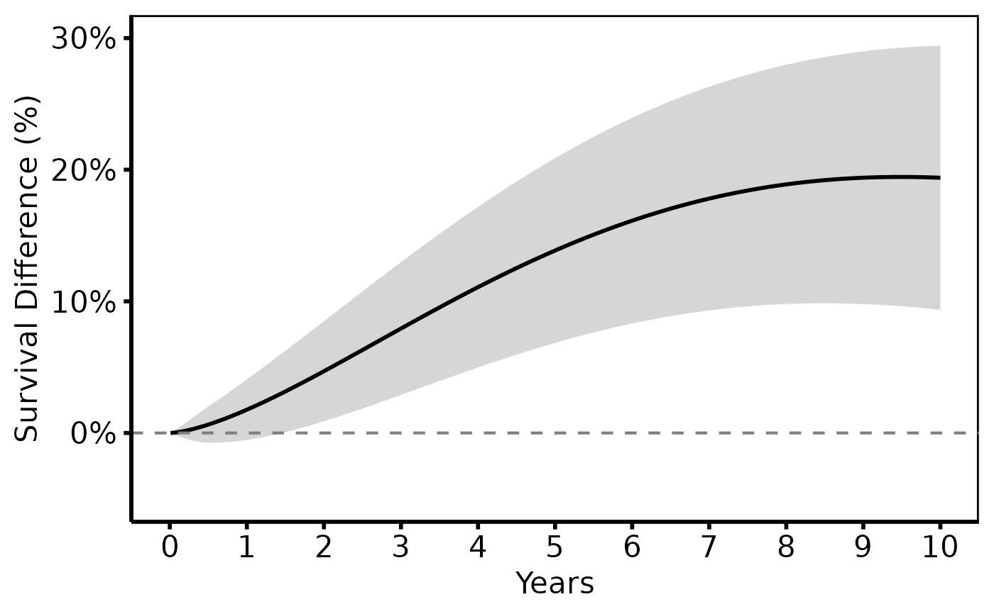
# --- (1) Single comparison: TF-TAVR vs TA-TAVR (tp.hp.dead.life-gained) --
survival_difference_plot(
diff_dat,
lower_col = "diff_lower",
upper_col = "diff_upper"
) +
scale_colour_manual(values = c("steelblue"), guide = "none") +
scale_fill_manual(values = c("steelblue"), guide = "none") +
geom_hline(yintercept = 0, linetype = "dashed", colour = "grey50") +
scale_x_continuous(limits = c(0, 10), breaks = 0:10) +
scale_y_continuous(limits = c(-5, 30),
labels = function(x) paste0(x, "%")) +
labs(x = "Years", y = "Survival Difference (%)") +
theme_hv_poster()
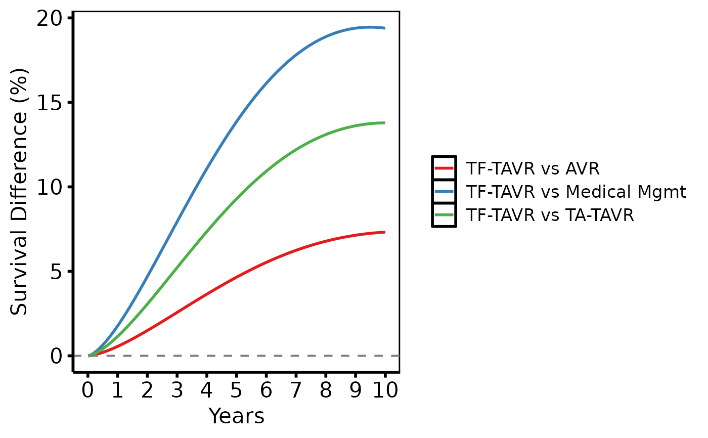
 # --- (2) Multiple treatment comparisons ----------------------------------
# Simulate three comparisons and combine (each row = one comparison)
d1 <- sample_survival_difference_data(
groups = c("Medical Mgmt" = 1.0, "TF-TAVR" = 0.70), seed = 1
)
d1$comparison <- "TF-TAVR vs Medical Mgmt"
d2 <- sample_survival_difference_data(
groups = c("TA-TAVR" = 0.90, "TF-TAVR" = 0.70), seed = 2
)
d2$comparison <- "TF-TAVR vs TA-TAVR"
d3 <- sample_survival_difference_data(
groups = c("AVR" = 0.80, "TF-TAVR" = 0.70), seed = 3
)
d3$comparison <- "TF-TAVR vs AVR"
dall <- rbind(d1, d2, d3)
survival_difference_plot(dall, group_col = "comparison") +
scale_colour_brewer(palette = "Set1", name = NULL) +
scale_fill_brewer(palette = "Set1", guide = "none") +
geom_hline(yintercept = 0, linetype = "dashed", colour = "grey50") +
scale_x_continuous(limits = c(0, 10), breaks = 0:10) +
labs(x = "Years", y = "Survival Difference (%)") +
theme_hv_poster()
# --- (2) Multiple treatment comparisons ----------------------------------
# Simulate three comparisons and combine (each row = one comparison)
d1 <- sample_survival_difference_data(
groups = c("Medical Mgmt" = 1.0, "TF-TAVR" = 0.70), seed = 1
)
d1$comparison <- "TF-TAVR vs Medical Mgmt"
d2 <- sample_survival_difference_data(
groups = c("TA-TAVR" = 0.90, "TF-TAVR" = 0.70), seed = 2
)
d2$comparison <- "TF-TAVR vs TA-TAVR"
d3 <- sample_survival_difference_data(
groups = c("AVR" = 0.80, "TF-TAVR" = 0.70), seed = 3
)
d3$comparison <- "TF-TAVR vs AVR"
dall <- rbind(d1, d2, d3)
survival_difference_plot(dall, group_col = "comparison") +
scale_colour_brewer(palette = "Set1", name = NULL) +
scale_fill_brewer(palette = "Set1", guide = "none") +
geom_hline(yintercept = 0, linetype = "dashed", colour = "grey50") +
scale_x_continuous(limits = c(0, 10), breaks = 0:10) +
labs(x = "Years", y = "Survival Difference (%)") +
theme_hv_poster()