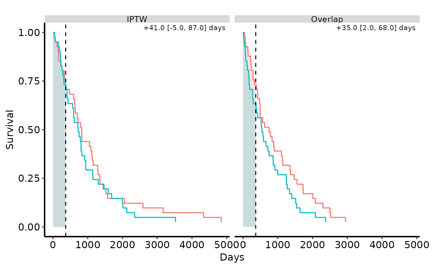
Prepare weighted Kaplan-Meier curves for an RMST figure

Validates the step-function curves behind an RMST analysis and returns an hv_rmst_curves object. Call plot.hv_rmst_curves() for a bare ggplot2 object with one facet per estimator and one step curve per arm. With tau, the area under each arm's curve up to tau is shaded (that area is the RMST) and a vertical line marks tau. With estimates, each facet is annotated with its RMST difference and interval.

Usage

hv_rmst_curves(
  curves,
  estimates = NULL,
  tau = NULL,
  facet = "estimator",
  arm = "arm",
  time = "time",
  surv = "surv",
  ...
)

Arguments

curves: A data frame of curve steps, or a ps_rmst object.
estimates: Optional data frame with the hv_rmst_contrast() columns (estimator, diff_days, lo_days, hi_days), used for the facet annotations. If NULL and curves is a ps_rmst-like object, its $tables$estimates is used when present. NULL otherwise: no annotation.
tau: Optional single positive number: the RMST horizon, on the same scale as time.
facet: Name of the column defining facets. Default "estimator". Factor levels set the facet order.
arm: Name of the arm column. Default "arm". A character column is ordered "treated", "control", then any other value.
time, surv: Names of the time and survival columns. Defaults "time" and "surv".
...: Ignored; present for S3 consistency.

Value

An object of class c("hv_rmst_curves", "hv_data"): a list with

$data: The curves data frame.
$meta: Named list: facet, arm, time, surv (column names), tau, facet_levels, arm_levels, n_missing.
$tables: shade: the staircase polygon under each curve up to tau (zero rows when tau is NULL); labels: one annotation per facet (zero rows when estimates is NULL).

Details

The input follows the tables$curves contract of hvtiRpropensity::ps_rmst(): columns estimator, arm ("treated" or "control"), time and surv, as right-continuous steps that start at time 0 with surv 1. hvtiRpropensity is not required: pass plain data frames, or the ps_rmst object itself as curves and its $tables$curves (and, when estimates is NULL, $tables$estimates) are read.

Examples

steps <- function(est, arm, rate) {
  t <- c(0, sort(round(stats::rexp(40, rate) * 365)))
  data.frame(estimator = est, arm = arm, time = t,
             surv = c(1, 1 - seq_len(40) / 41))
}
set.seed(1)
curves <- rbind(
  steps("IPTW", "treated", 1 / 3), steps("IPTW", "control", 1 / 2),
  steps("Overlap", "treated", 1 / 3), steps("Overlap", "control", 1 / 2)
)
est <- data.frame(estimator = c("IPTW", "Overlap"),
                  diff_days = c(41, 35), lo_days = c(-5, 2), hi_days = c(87, 68))

rc <- hv_rmst_curves(curves, estimates = est, tau = 365)
rc
#> <hv_rmst_curves>
#>   Facets  : 2 (IPTW, Overlap)
#>   Arms    : treated, control
#>   Tau     : 365
#>   Labels  : RMST difference

plot(rc) +
  ggplot2::labs(x = "Days", y = "Survival") +
  theme_hv_manuscript()