p    <- plot(hv_survival(sample_survival_data(n = 500, seed = 42)))
p_ms <- p + theme_hv_manuscript(base_size = 12)
p_ms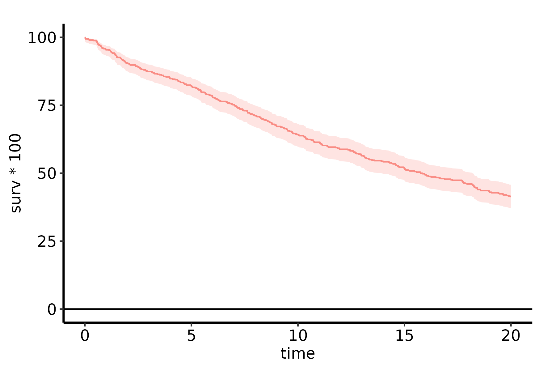
Journals impose hard constraints on figures: a fixed column or page width, a maximum height, and a vector format (PDF/EPS) so type and lines stay crisp at print resolution. The trap is that two figures saved at the same ggsave() dimensions rarely share the same data region: a longer axis label or a wider legend steals space from the panel, so the plotting area drifts from figure to figure. theme_hv_manuscript() sets a print-appropriate base size, and hv_ggsave_dims() pins the panel content area to a constant rectangle across a figure set.
theme_hv_manuscript() uses a 12 pt base on a white background, sized for the final printed page rather than the screen.
p <- plot(hv_survival(sample_survival_data(n = 500, seed = 42)))
p_ms <- p + theme_hv_manuscript(base_size = 12)
p_msFor most figures the quickest path is save_manuscript(), which writes a finished plot at the house manuscript size, 6 × 4 inches, in one call.
save_manuscript(p_ms, "trends_manuscript.pdf")It is the manuscript counterpart of save_ppt(): it fixes the output geometry, not the theme, so the 12 pt type comes from the theme_hv_manuscript() you have already applied. Override the size when a journal asks for it, for a single column, say save_manuscript(p_ms, "fig.pdf", width = 3.5, height = 3), and pass a device when you need font embedding, with the caveat below. The chunks in this section are eval: false because each writes a binary file.
save_manuscript(), like ggsave(), fixes the file dimensions but lets the panel float inside them. When you need the panel content area identical across several figures, so the data regions line up regardless of how much room each plot’s axis labels take, hv_ggsave_dims() inverts the problem: you specify the panel content area you want (the rectangular bounding box of the gtable cells tagged panel) and it returns the width/height/units such that ggsave() yields exactly that panel size, expanding the file to absorb axes, titles, and any remaining chrome. The result is a named list shaped to splat directly into ggsave() via do.call().
dims <- hv_ggsave_dims(p_ms, width = 6, height = 4, units = "in")

do.call(
  ggsave,
  c(
    list(filename = "trends_manuscript.pdf", plot = p_ms,
         device = grDevices::quartz, type = "pdf"),
    dims
  )
)
The device matters, and the usual recommendation has a failure mode worth knowing. cairo_pdf embeds fonts and renders transparency and custom typefaces correctly, where the base pdf device substitutes them. But on a Mac without XQuartz it warns “failed to load cairo DLL”, returns without error, and writes no file. Measured on the machine that builds this book: ggsave() reported success and the target PDF did not exist. A silent no-op is worse than a failure you can see, so check that the file appeared before assuming a cairo export worked.
The quartz device above is the macOS answer: part of the operating system, nothing to install, fonts embedded, full Unicode range. It is what this book’s own PDF build uses, for the same reason. On Linux, cairo_pdf with a working cairo is the right call. The chunk is eval: false because it writes a binary file; the code is shown, not run during the book build.
For multi-panel figure sets where the data region must be identical across several PDFs regardless of label length, call hv_ggsave_dims() with the same width/height for each figure. Its slide-layout analogue, hv_ph_location(), computes officer::ph_location() coordinates so a panel lands at the same slide position in a deck.
save_ppt() writes the plot into a PowerPoint slide as editable DrawingML vector graphics via the officer and rvg packages: shapes, lines, and text remain selectable in PowerPoint, so co-authors can re-label or recolor without round-tripping back to R. It appends a slide to a template .pptx rather than overwriting it.
template <- system.file("ClevelandClinic.pptx", package = "hvtiPlotR")

p_ppt <- p + theme_hv_ppt_dark()

save_ppt(
  object       = p_ppt,
  template     = template,
  powerpoint   = "trends_slides.pptx",
  slide_titles = "Overall Survival",
  width        = 10.1,
  height       = 5.8
)
This chunk is eval: false because it writes a .pptx file. To anchor the panel content area at identical slide coordinates across a multi-slide deck (useful when axis-label widths differ between plots), pass panel_box = list(width, height, left, top); save_ppt() delegates to hv_ph_location() per slide.