Postoperative risk rarely stays constant. It may be high immediately after an operation, settle to a low background rate after recovery, then rise again as the patient and the repair age. A Kaplan-Meier curve tells us how much survival remains. An additive hazard model asks the companion clinical question: which early, constant, or late process is contributing risk at each time?
Begin with the empirical curves. They are the evidence for choosing a parametric shape, not decoration added after the model is fit. If the empirical hazard falls sharply and then flattens, one monotone Weibull may be a useful summary. If it shows distinct regions, fit those phases explicitly and check the total curve against the empirical estimate.
TemporalHazard(Ehrlinger 2026) is the maintained R implementation of the Blackstone, Naftel, and Turner additive hazard model. It replaces the historical SAS/C HAZARD workflow in this recipe. We fit and inspect the R object here; the prediction chapter then turns it into curves.
22.2 The data it needs
Both examples use public data bundled with TemporalHazard. cabgkul contains 5,880 primary isolated CABG patients, with follow-up in months and a death indicator. avc contains 310 patients after atrioventricular canal repair and supports the two clinically identifiable phases used below. No patient extract is needed to run either recipe.
hzr_kaplan() estimates survival and hzr_nelson() estimates cumulative hazard from the same subject-level records. Build both objects before choosing a distribution, then inspect the columns that will be plotted.
km <-hzr_kaplan(cabgkul$int_dead, cabgkul$dead)na <-hzr_nelson(cabgkul$int_dead, cabgkul$dead)head(as.data.frame(km)[c("time", "n_risk", "n_event", "survival","cl_lower", "cl_upper")])
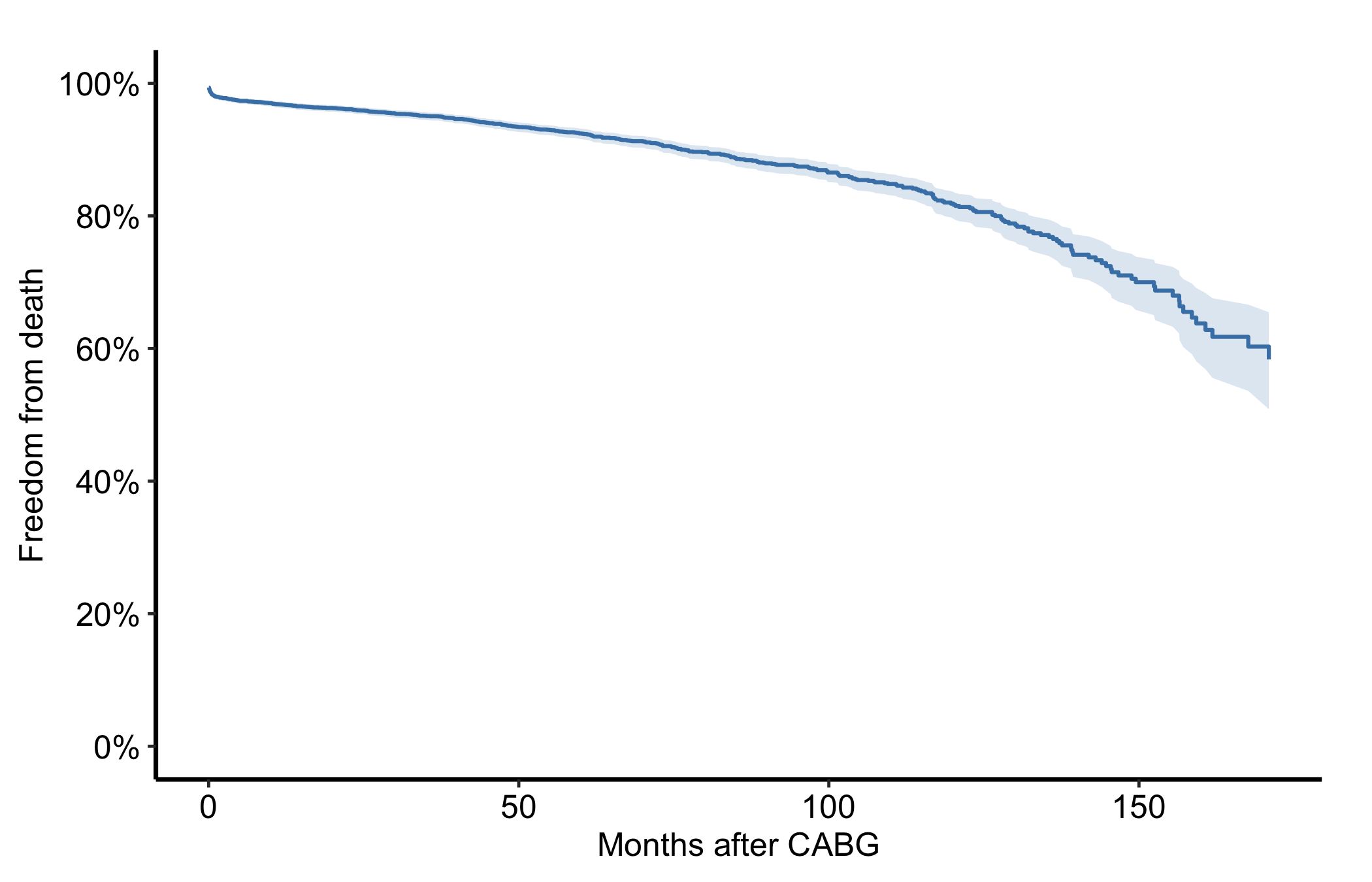
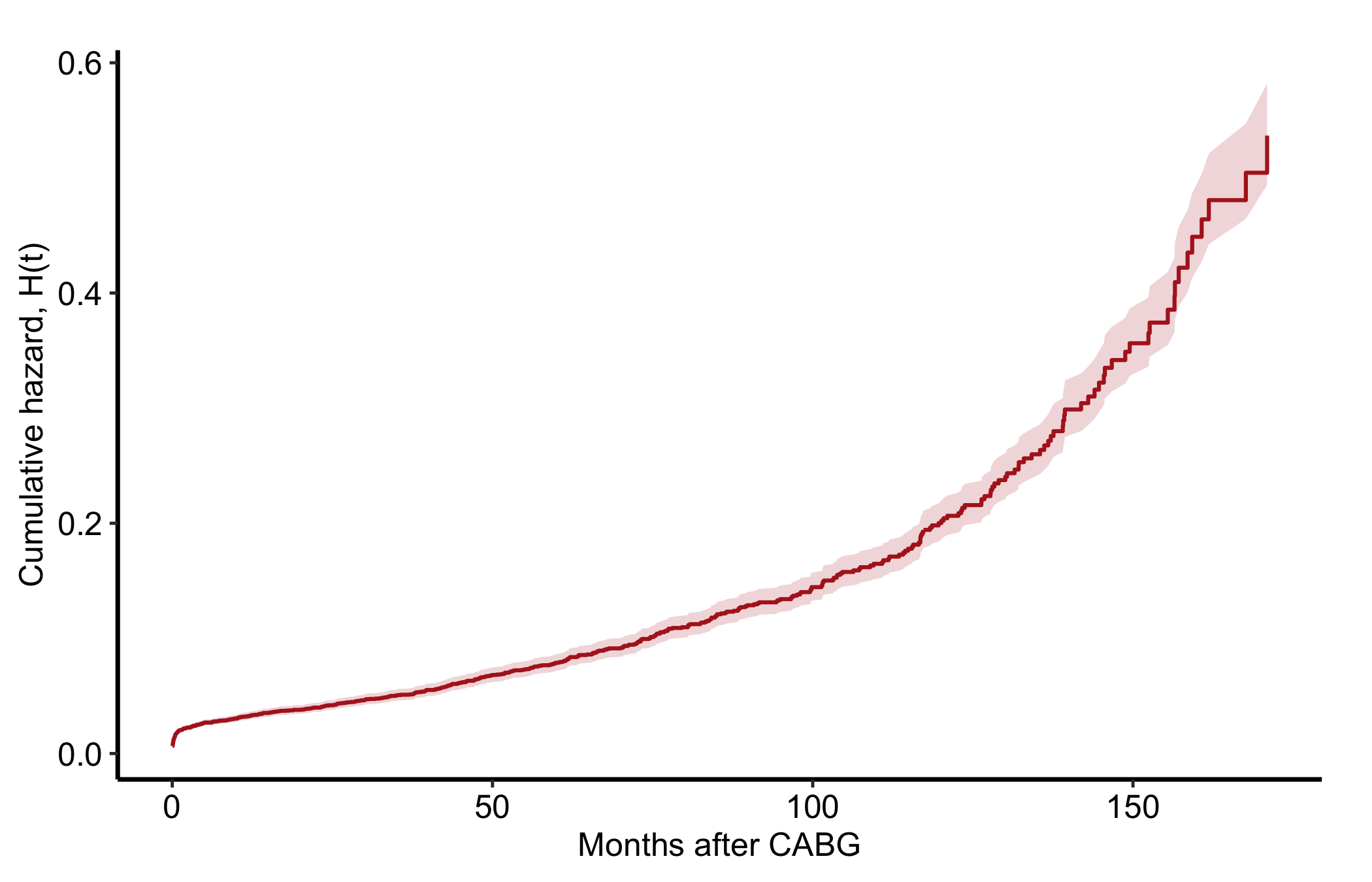
The Kaplan-Meier panel shows the surviving fraction. The Nelson-Aalen panel turns the same follow-up into accumulated event intensity. Its local slope is the empirical clue to the hazard shape: changing slope means the instantaneous risk is changing with time.
Figure 22.1: Empirical Kaplan-Meier survival for the CABG cohort, with logit-transform 95% confidence limits. The steel-blue step line is the survival estimate and the light blue band its 95% confidence limits.
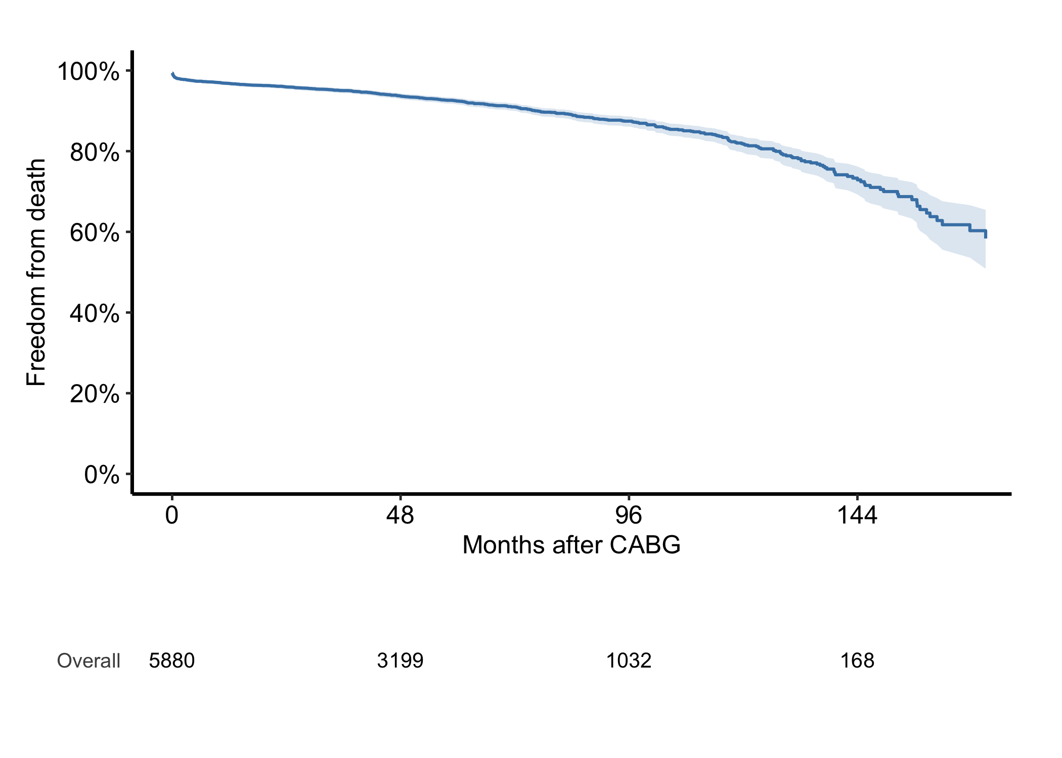
The curve alone does not say how much cohort is left behind each part of it, and by the late follow-up here that is most of what a reader needs. hv_atrisk() counts the risk set at times you choose and hv_atrisk_compose() stacks it under the curve on a matched axis. It reads the same subject-level records hzr_kaplan() did, which is what makes the counts belong to this curve rather than to a cohort that happens to resemble it.
# Free size: curve stacked over a numbers-at-risk table.curve <-ggplot(km, aes(time, survival *100)) +geom_ribbon(aes(ymin = cl_lower *100, ymax = cl_upper *100),fill ="steelblue", alpha =0.18) +geom_step(colour ="steelblue", linewidth =0.7) +scale_y_continuous(limits =c(0, 100), breaks =seq(0, 100, 20),labels =function(x) paste0(x, "%")) +scale_x_continuous(breaks =seq(0, 144, 48)) +coord_cartesian(xlim =c(0, 168)) +labs(x ="Months after CABG", y ="Freedom from death") +theme_hv_manuscript(base_size =12)risk_panel <-hv_atrisk(cabgkul, time ="int_dead", status ="dead",report_times =seq(0, 144, 48))hv_atrisk_compose(curve, risk_panel)
Figure 22.2: The same Kaplan-Meier estimate with an aligned numbers-at-risk table, showing how little cohort supports the late tail. The steel-blue step line is the survival estimate, the light blue band its 95% confidence limits, and the black numbers below the curve the patients still at risk.
Read the two together. Freedom from death is around 60% at the right-hand edge, but 168 patients remain at twelve years against 5,880 at the start, so that part of the curve rests on a small and increasingly selected group. The widening confidence band says the same thing; the counts say it in a number a reviewer can check. Choose report_times that a clinical reader thinks in, and stop them where the cohort still supports an estimate rather than running them to the last observed event.
Figure 22.3: Empirical Nelson-Aalen cumulative hazard for the CABG cohort, with lognormal 95% confidence limits. The firebrick-red step line is the cumulative hazard estimate and the light red band its 95% confidence limits.
22.4 Fit a reviewed Weibull model
Now fit the simple parametric description. The reviewed starting vector has a scale and shape value; it is an optimizer starting point, not a result to report. The estimates belong to the fitted object returned by hazard().
fit <-hazard(time = cabgkul$int_dead,status = cabgkul$dead,theta =c(0.01, 1),dist ="weibull",fit =TRUE)summary(fit)
hazard model summary
  observations: 5880
  predictors:   0
  dist:         weibull
  engine:       native-r-m2
  converged:    TRUE
  gradient:     relative 9.45e-09 (SAS/C requires <= 6.06e-06; met, nlm code 1)
  log-lik:      -3935.72
  Not done in this run: none
  evaluations: fn=37, gr=9
  message:      continued with nlm() for 3 iterations (code 1)

Coefficients:
       estimate    std_error   z_stat       p_value
mu 0.0003615964 6.018412e-05  6.00817  1.876291e-09
nu 0.5945264679 2.346396e-02 25.33786 1.222989e-141
The fitted Weibull shape is below 1, so its hazard declines with time. That is consistent with an early postoperative component, but the single curve cannot separate an early decline from a continuing background rate. Thus we treat it as a compact population summary and keep the empirical panels beside it as the fit check.
22.5 Fit the early and constant phases
The AVC data have a clear early risk period and a much lower continuing rate. We represent those with an early CDF phase plus a constant phase. The early shape values below are the reviewed package example; fixed = "shapes" holds them fixed while the model estimates the scale of each phase. We do not invent new starting values.
Multiphase hazard model (2 phases)
  observations: 305
  predictors:   0
  dist:         multiphase
  phase 1:      early - cdf (early risk)
  phase 2:      constant - constant (flat rate)
  engine:       native-r-m2
  converged:    TRUE
  gradient:     relative 1.27e-09 (SAS/C requires <= 6.06e-06; met, nlm code 1)
  log-lik:      -228.029
  Not done in this run: none
  evaluations: fn=26, gr=3
  message:      continued with nlm() for 1 iterations (code 1)

Coefficients (internal scale):

  Phase: early (cdf)
               estimate std_error    z_stat     p_value
  log_mu     -1.4132735 0.1290435 -10.95192 6.50568e-28
  log_t_half -0.6931472        NA        NA          NA
  nu          1.0000000        NA        NA          NA
  m           1.0000000        NA        NA          NA

  Phase: constant (constant)
          estimate std_error    z_stat      p_value
  log_mu -7.609476 0.4495826 -16.92564 2.911456e-64
Inspect convergence separately from the coefficient table. A populated summary is not enough: the optimizer must converge, and the covariance calculation must be positive definite for the free parameters.
At 0.5 months, the evaluated early hazard contribution is much higher than the constant contribution on the same per-month scale. It then declines, while the constant contribution remains flat and continues to accumulate through late follow-up. The two phases overlap and add; the model does not switch from one to the other at 0.5 months. For this bounded early CDF phase, t_half = 0.5 means that half of the early phase’s eventual cumulative-hazard contribution has accumulated by 0.5 months.
22.6 Read convergence warnings before reading the curves
A multiphase model can return numbers even when the data do not identify the requested phases. Stop and simplify the model when any of these occur:
fit$fit$converged is FALSE, especially after the iteration limit.
The covariance matrix is unavailable or fit$fit$pd is FALSE.
A free parameter has an enormous standard error, or a fitted phase scale is effectively zero.
Two phases trace nearly the same shape and compete to explain the same events.
Those are model warnings, not requests for a larger maxit. First ask whether the empirical curve contains the phase at all. Fixing reviewed shape parameters reduces the number of quantities the data must identify; adding an unsupported late phase does the opposite.