Every survival recipe so far has assumed one row per patient. Baseline creatinine, baseline ejection fraction, the covariate values as they stood on day zero, and a single follow-up time. That assumption is usually a simplification we accept, and sometimes it is the thing that ruins the analysis. A patient on temporary mechanical support has a risk profile that changes week by week. Freezing them at their admission values throws away the part of the record that was doing the work.
A Random Hazard Forest takes the counting-process form instead: several rows per patient, each covering an interval of follow-up, with covariates allowed to change between intervals. The forest sees what changed and when, so its predictions can be read on the same clinical timeline as the measurements.
Reach for this when the exposure is time-varying and the timing matters, not just its presence. Support escalation, a therapy that starts partway through admission, a lab that drifts. If your predictors are genuinely fixed at baseline, the survival and forest prediction recipes are the simpler and better fit, and nothing here improves on them for that case.
This chapter reads a fitted forest. Growing one is the job of randomForestRHF(Ishwaran and Kogalur 2026); the reading is done by ggRandomForests(Ehrlinger 2026). The boundary between the two is worth keeping straight, so it has its own section near the end.
34.2 The data it needs
The counting-process layout gives each patient one row per interval (start, stop], and event records whether the event happened at that interval’s right endpoint. We work from the reviewed bundle that ships with the ggRandomForests article, so the chapter renders without refitting.
Read down the xtd column, then consider x.1, which is not shown because it never moves. That is the whole distinction: xtd is the time-varying covariate and the x.1 through x.10 columns are fixed at baseline. A counting-process frame carries both, and the forest treats them differently only because the data says they behave differently.
The rule that makes this legitimate is predictability: the value used at time t must be known just before the event decision at t. A lab drawn after an interval ends cannot be copied backward into it. In this simulation xtd is a continuous function of stop and the subject’s own fixed covariates, so its value at stop is also its left-hand limit there, and it is available for the interval ending at that time.
That is not a technicality. Copying a later measurement backward is how a model learns to predict an event from evidence produced by the event, and it is the most common way a time-varying analysis flatters itself. The no-lookahead routing is enforced by randomForestRHF::rhf() when the forest is grown, not by anything in this chapter.
records_per_subject <-as.integer(table(rhf_data$id))events_by_subject <-tapply(rhf_data$event, rhf_data$id, max)data.frame(measure =c("Subjects", "Counting-process records", "Records per subject","Subjects with an event"),value =c(length(unique(rhf_data$id)),nrow(rhf_data),sprintf("%d to %d (median %g)", min(records_per_subject),max(records_per_subject), stats::median(records_per_subject)),sum(events_by_subject))) |> knitr::kable(col.names =c("Measure", "Value"))
Measure
Value
Subjects
500
Counting-process records
2598
Records per subject
2 to 7 (median 5)
Subjects with an event
427
34.3 Where these fitted objects came from
The bundle holds the fit and three upstream results that are far too slow to recompute on every render. The calls that produced it are shown but not run.
Supplying the saved results to the extractors is the pattern to copy for any analysis you expect to revisit. Each gg_* function below will compute its own input when you do not hand it one, which is convenient once and expensive every time after that.
34.4 Read the hazard over time
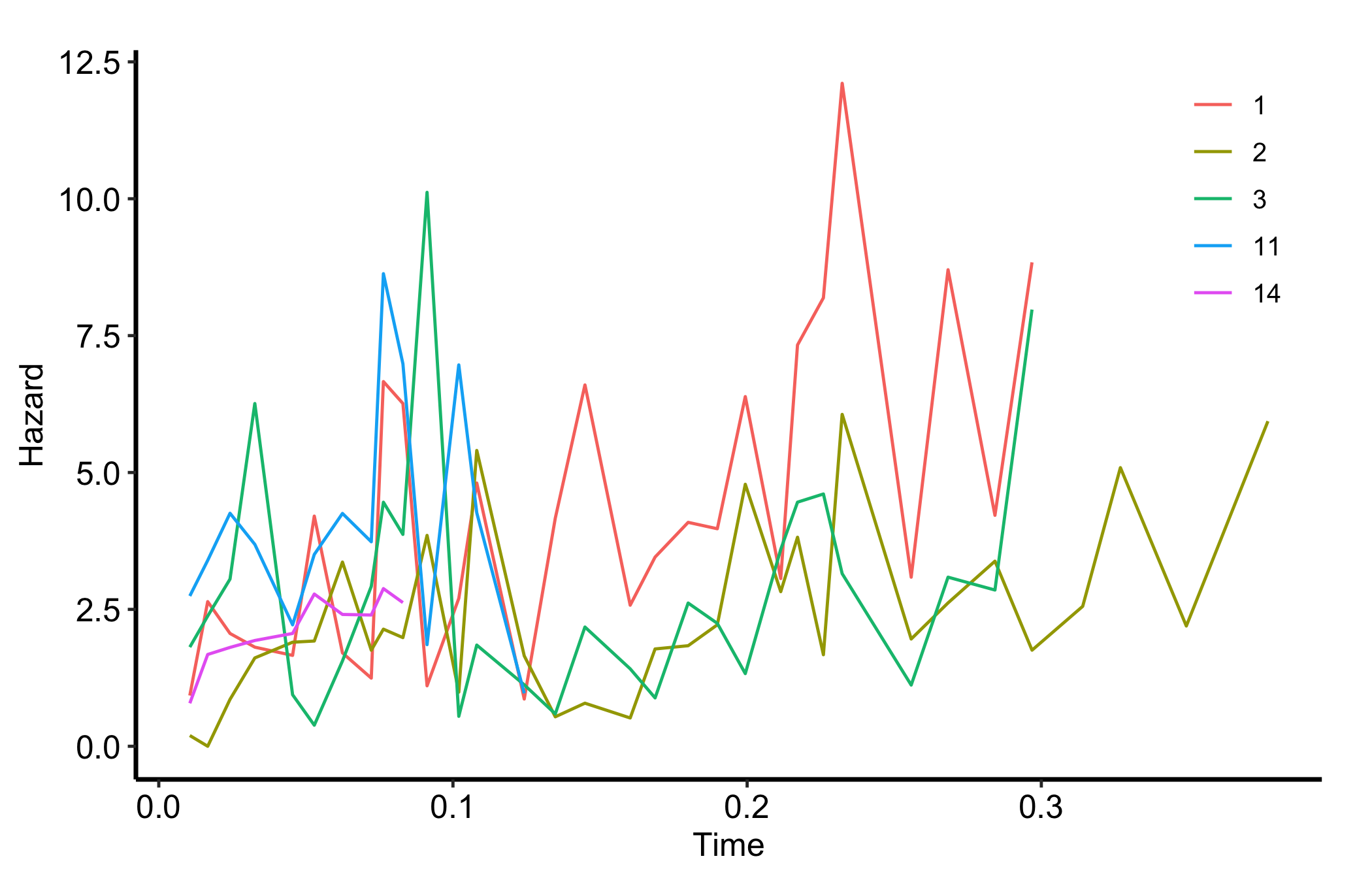
gg_rhf() pulls both the pointwise hazard and the cumulative hazard into one tidy frame, one row per subject per point on the forest’s working time grid.
Figure 34.1: Out-of-bag pointwise hazard for five of six requested subjects, each curve ending where that subject’s follow-up ends; subject 22 has no grid point inside its records and so draws nothing. Each solid line is one subject, one color per subject, as in the legend.
All four house themes set legend.position = "none" on purpose: a CORR figure carries no legend, and groups get named on the panel instead, which is the recipe in Section 37.4. This figure is the documented exception rather than a departure from it. The six lines are simulated subject identifiers, not clinical groups, so there is nothing meaningful to annotate beside each curve, and legends is explicit that you want a key whenever the grouping is not already named on the panel. hv_legend_inside() is how you add one without giving up panel width: apply it after the theme so its position wins, and it anchors the key in whichever corner the data leave emptiest.
Hazard here is a local event rate: a high point says events are occurring at a high instantaneous rate among the subjects still at risk around that time. It is not the probability that this subject has the event then, and neither its height nor its scale should be reported as a percentage. We plot six subjects, not all of them: the extracted object holds a curve for every subject, and a panel becomes unreadable long before it shows them all.
The curves stop at different places, and that is deliberate rather than missing data. From version 2.0.0, randomForestRHF::rhf() returns a hazard only where a grid point falls inside one of that subject’s supplied (start, stop] records, and NA in the gaps and after the final stop. Each line therefore covers the range the forest was asked about.
Count the legend and you get five, though we asked for six. Subject 22 has no grid point inside any of its records, so every one of its hazard values is NA and it draws nothing at all. That is the masking rule taken to its limit rather than a plotting failure, and a requested subject can disappear from this panel entirely. It comes back in the next one.
34.4.1 Cumulative hazard accumulates the local rates
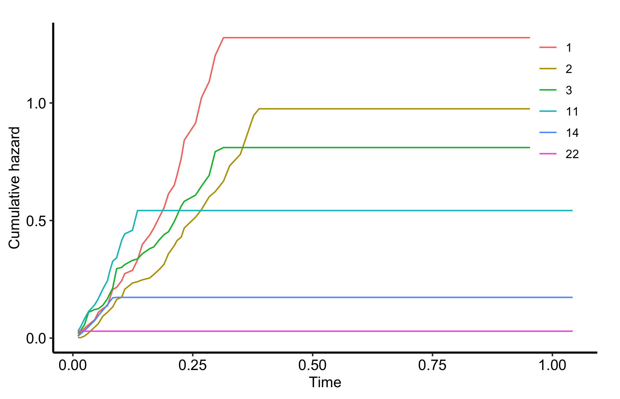
The same object carries the cumulative hazard. Set hazard.only = FALSE to draw it.
Figure 34.2: Cumulative hazard for the same six subjects, all present this time, drawn across the whole grid because it accumulates interval overlap rather than being masked outside the records. Each solid line is one subject, one color per subject, as in the legend.
Cumulative hazard is not masked the way the pointwise hazard is. It accumulates the exact overlap between the working grid and the supplied records, so it stays flat through a gap instead of going missing, and every grid point is drawn. Subject 22 is back, as a flat line just above zero: it accumulated almost no hazard, which is a different statement from having none to report.
The practical consequence is small and easy to trip over: if you summarise the hazard column yourself, pass na.rm = TRUE. Counting subjects off a hazard panel will also undercount them.
34.5 Does discrimination hold up over time?
A single concordance number for the whole of follow-up hides the thing you usually want to know, which is whether the model still separates patients late as well as it did early. Time-varying AUC answers that, and which AUC you want depends on the question.
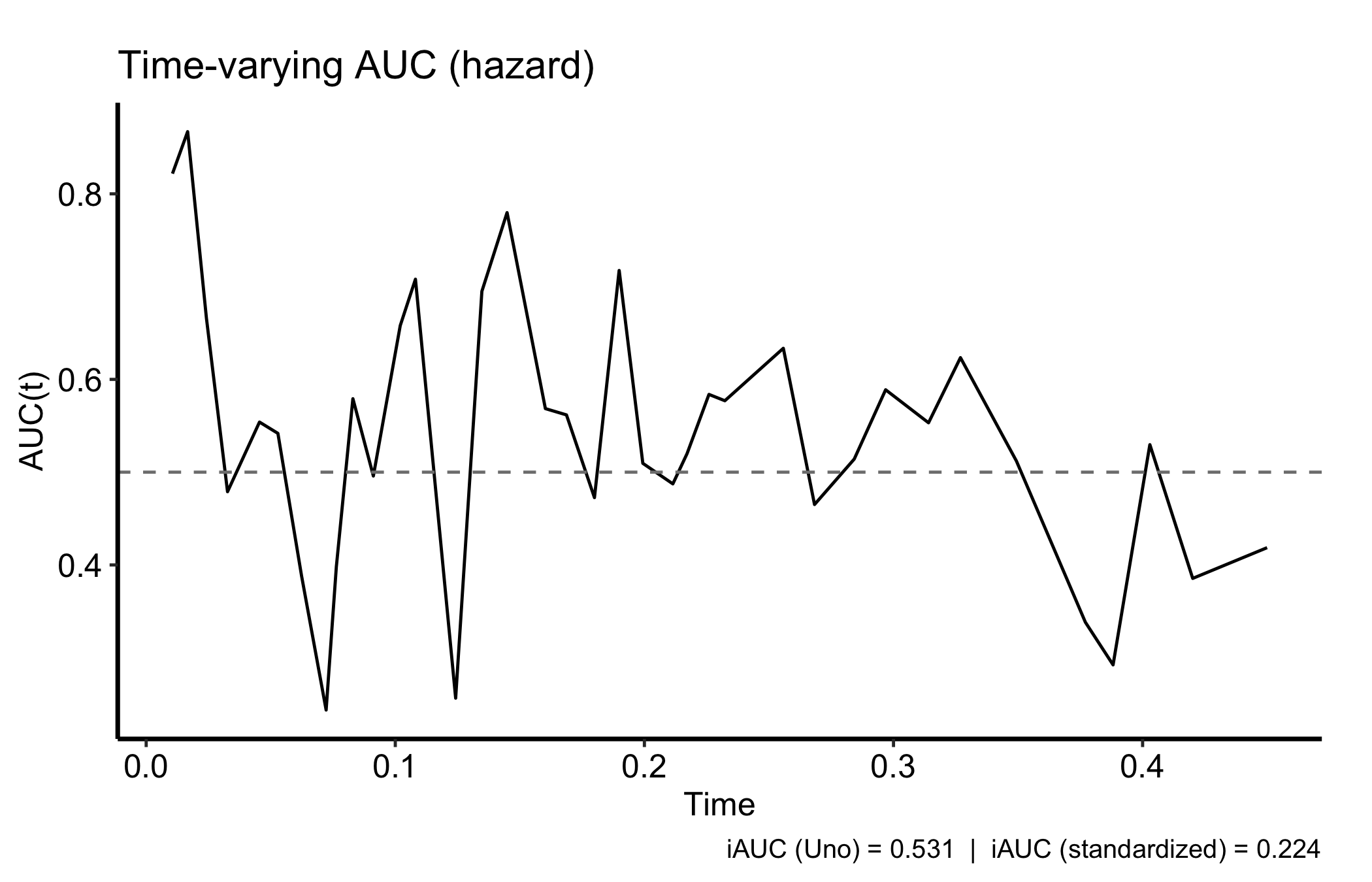
gg_auct() with marker = "haz" gives the incident/dynamic definition: does a subject who has the event near time t rank above a subject in the risk set at t? That is a question about local failures, so it uses the local hazard marker.
Figure 34.3: Incident/dynamic time-varying AUC from the saved calculation, with the 0.5 chance line for reference. The solid black line is the AUC at each time and the dashed grey horizontal line the 0.5 chance level.
The saved curve has a Uno integrated AUC of 0.531, and its finite values run from 0.244 to 0.867. AUC is a ranking probability on a 0 to 1 scale, so 0.5 is the chance reference drawn on the panel. This calculation was not bootstrapped, so there is no confidence ribbon; supply a bootstrapped auct_fit and one appears.
The companion definition, cumulative/dynamic, asks whether a subject who has had the event by a horizon ranks above one still event-free at that horizon, and its matching marker is cumulative hazard. It targets a different quantity rather than a better version of the same one. On in-sample data of this shape it is currently awkward to read, because holding the cumulative hazard flat after follow-up ends makes it track observation length as well as risk. Reach for it on genuinely out-of-sample predictions, and read the incident/dynamic curve here.
34.6 Which variables matter, and when?
Ordinary variable importance gives one number per predictor for the whole study. With time-varying data that is the wrong shape: a covariate can dominate early and stop mattering entirely once patients are past the risky window.
# Free size: one row per variable and one column per time window, so the height grows with the variable list.rhf_priority <-gg_rhf_importance(bundle$fit, importance_fit = bundle$importance)windows <-unique(as.data.frame(rhf_priority)[, c("time_window", "start", "stop")])windows <- windows[order(windows$start), ]window_labels <-setNames(sprintf("%.2f to %.2f", windows$start, windows$stop), windows$time_window)plot(rhf_priority) +scale_x_discrete(labels = window_labels) +theme_hv_manuscript(base_size =12) +theme(legend.position ="right", plot.margin =margin(l =80))
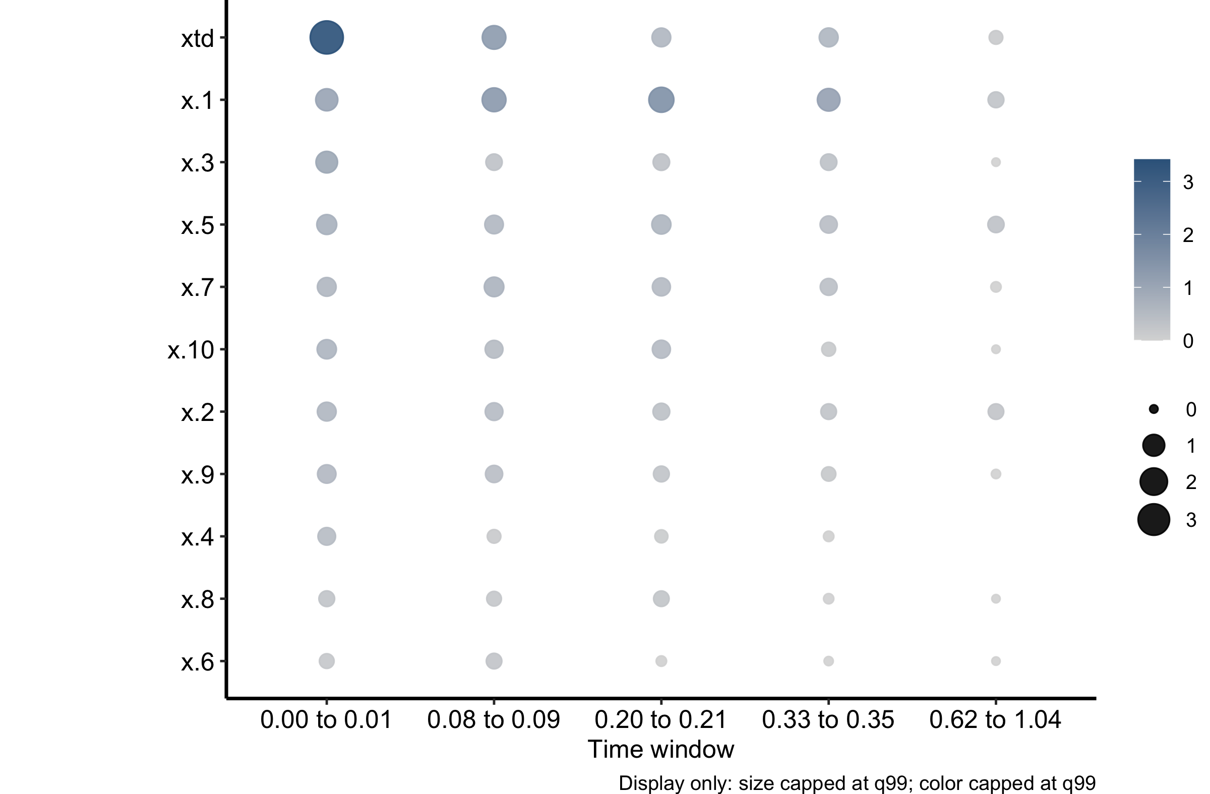
Figure 34.4: Time-localized variable priority across five time windows, with point size and color showing the same priority value. Each filled circle is one variable in one window; larger, darker steel-blue circles mark higher priority and small light grey circles the lowest.
Two adjustments earn their place here. The window labels arrive as full-precision interval strings such as (0.00000000, 0.01055113], and five of those overlap into an unreadable band along the axis, so we rebuild them from the start and stop columns at two decimals. And the legend goes back on the outside rather than inside: point size and colour both encode priority, so the key is a continuous scale rather than a short list of series, and dropping it into the panel would sit on top of the matrix it explains.
RHF priority is a time-local rule-release contrast. Within a window it compares the fitted working response for a rule against its near-miss set, and asks how much that response moves when rules involving a variable are released. Larger nonnegative values mean a larger contrast.
Read that sentence again before reporting anything from this figure, because of what it does not say. Priority does not tell you the direction of an effect, so it never licenses “higher xtd raises hazard”. It is not a z-score, not a p-value, and carries no selection threshold. It ranks, and that is all.
In this simulation xtd carries the largest early-window value while x.1 leads several later windows, which is exactly the pattern a single whole-study importance number would have averaged away. The number at risk also falls from 779 to 32 across the five windows, so the late-window comparisons rest on much less information than the early ones. Any window-to-window story should be told with that in view.
34.7 Which tree size did the search pick?
gg_tune_rhf() reads a completed tuning path. It never reruns the search, and it preserves the upstream evaluation order, so the connecting line follows the order candidates were tried rather than a tidied-up sort.
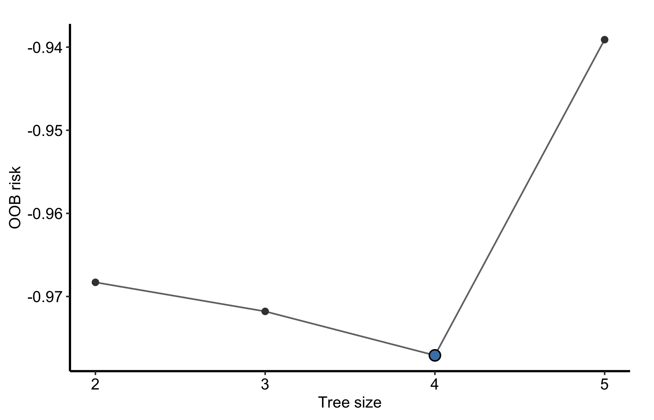
Figure 34.5: Out-of-bag risk tuning path, with the emphasized point marking the size the upstream search selected. Small dark grey filled circles joined by a grey solid line mark each tree size tried, and the larger steel-blue circle with a black outline marks the selected size.
The risk search evaluated sizes 2, 3, 4, 5 and selected 4, where mean out-of-bag risk was smallest. The saved risk path carries no standard-error field, and gg_tune_rhf() sets se to missing rather than inventing uncertainty, so this plot has no ribbon.
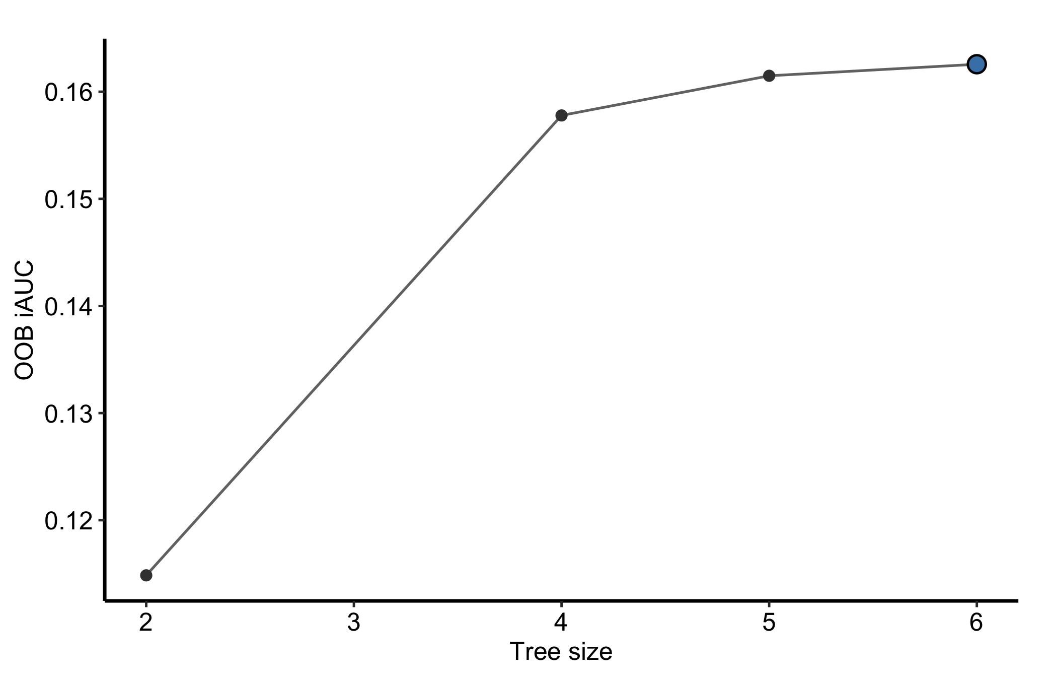
Figure 34.6: The same tuning display for the integrated-AUC search, which selected a different tree size than the risk search did. Small dark grey filled circles joined by a grey solid line mark each tree size tried, and the larger steel-blue circle with a black outline marks the selected size.
This search evaluated 2, 4, 5, 6 and selected 6, where out-of-bag iAUC was largest. The two searches choose differently, and that is the useful part. Risk and discrimination are not the same objective, and a tree size that minimises one need not maximise the other. Say which criterion you tuned on when you report a size. This path has 0 finite standard errors, so again no ribbon.
34.8 What each extractor returns
Each gg_* function returns a data frame you can work with directly, which matters when a figure is not the deliverable.
Function
One row per
Key columns
gg_rhf()
subject and grid time
id, time, hazard, chf, source
gg_auct()
grid time
time, auc, se, lower, upper, marker, plus an iauc attribute
gg_rhf_importance()
variable and time window
variable, time_window, time, n_risk, n_rules, priority
gg_tune_rhf()
candidate tree size
treesize, metric, value, se, selected
The iauc attribute on gg_auct() is the one people miss. It carries the Uno and standardized integrated AUC, and attr(x, "iauc") is how you reach it for a table.
34.9 Where ggRandomForests ends and randomForestRHF begins
This chapter draws pictures of decisions made elsewhere. Knowing which package owns what keeps an upstream modelling choice from being read as a plotting defect.
randomForestRHF owns the model. It sets the working time grid, applies the no-lookahead routing, decides that the pointwise hazard exists only inside supplied records, computes the AUC under its chosen definition, evaluates variable priority, and runs the tuning search. From 2.0.0 it also defaults to adaptive hazard aggregation, which shifts fitted values relative to earlier versions.
ggRandomForests reads those results and tidies them. It passes the NA mask through unchanged, drops those points at draw time so a curve ends with its subject’s follow-up, preserves the upstream tuning order, and declines to fabricate standard errors the upstream object does not carry.
So a hazard curve that stops early, a missing late-window priority point, and a tuning plot with no ribbon are all faithful reports of the fitted object. If you want different behaviour there, the change belongs upstream.
34.10 Pitfalls
A counting-process frame is not a wide longitudinal frame. One row per interval, with (start, stop] half-open so consecutive intervals do not double-count the boundary. Reshaping one repeated-measures column per visit into start/stop rows is the step most likely to go wrong, and it goes wrong silently.
Predictability is the assumption that carries the analysis. A value used at time t must be knowable just before t. Carrying a later lab backward into an earlier interval produces a model that predicts events from their own consequences, and reports excellent discrimination while doing it.
A subject can vanish from a hazard panel. If no grid point falls inside any of its records, every hazard value is NA and the line is not drawn. The subject is still in the extracted frame and still appears in the cumulative-hazard panel. Never read the number of lines on a hazard figure as the number of subjects you asked for.
Hazard is a rate, not a probability. Do not report a hazard height as a percentage, and do not compare hazard heights across figures drawn on different grids.
Priority ranks; it does not direct.gg_rhf_importance() says a variable mattered in a window, never which way it pushed. Pair it with a dependence view before writing a direction into a manuscript.
Say which criterion you tuned on. The risk and iAUC searches selected different tree sizes on the same data. A reported tree size is uninterpretable without its objective.
Supply the saved upstream objects.gg_auct(), gg_rhf_importance() and gg_tune_rhf() will each compute their input when you omit it. That is fine once and painful in a document you re-render, which is why this chapter passes auct_fit, importance_fit, and a completed tuning path.
The house themes suppress legends deliberately, so add one deliberately. All four theme_hv_*() functions set legend.position = "none" because a CORR figure names its groups on the panel rather than in a margin key. When the grouping genuinely cannot be named that way, restore the key after the theme: hv_legend_inside() for a handful of series, an explicit legend.position for a continuous scale that would occlude the data if placed inside.
Late windows rest on fewer patients. The number at risk falls sharply across the importance windows here. Read late-window contrasts with that in mind rather than as equals of the early ones.