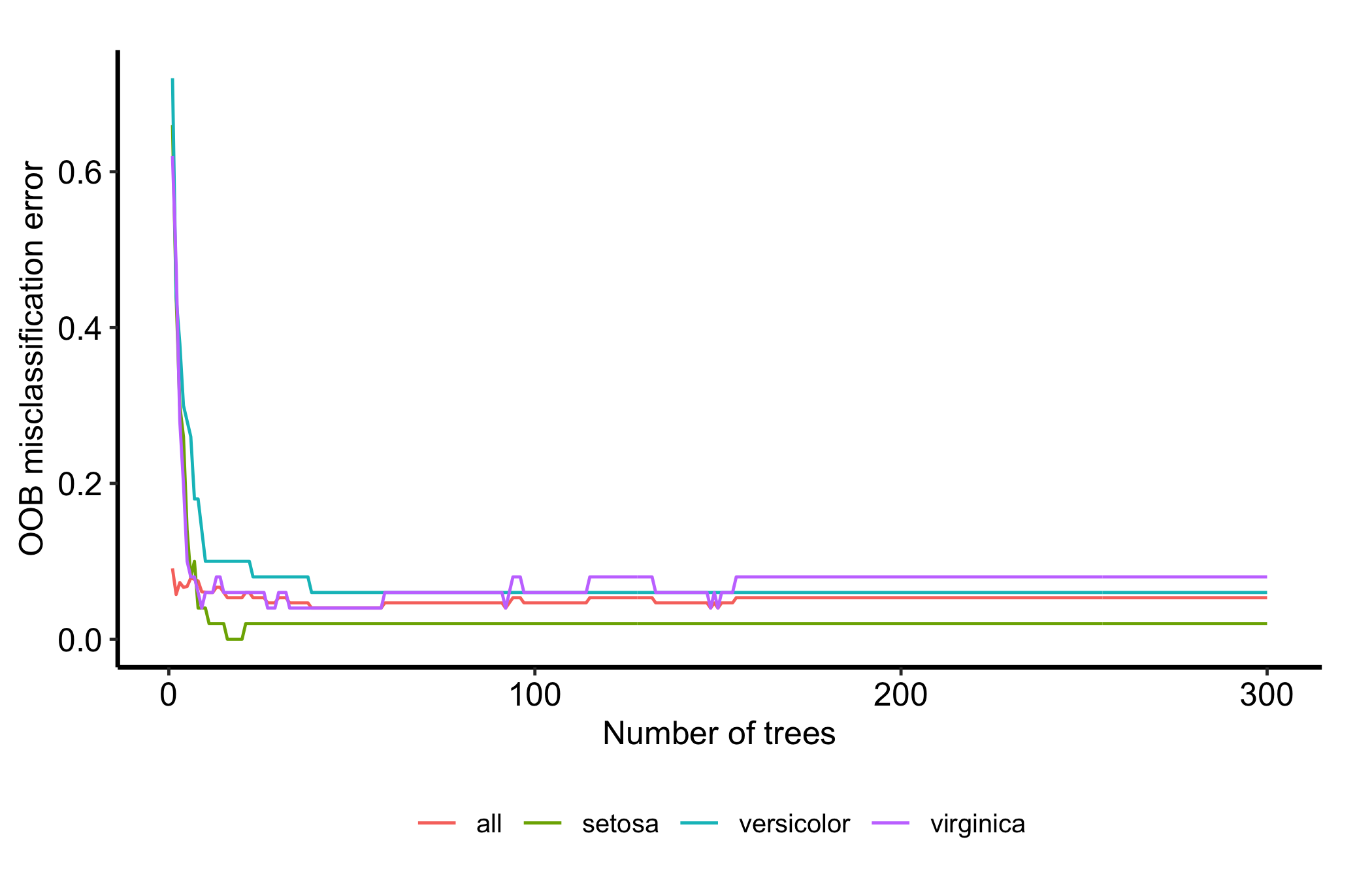
A forest prediction is an average over trees, so our first question is whether that average has stopped changing materially as trees are added. gg_error() shows the cumulative out-of-bag (OOB) error recorded while the forest grew. Use it before reading an importance ranking or a predicted curve.
The display is a tree-count diagnostic. A roughly level tail says the fitted forest is no longer sensitive to adding a few more trees. It does not prove that the model transports to another population, that its predictors are causal, or even that its absolute prediction error is acceptable.
26.2 Fit a bounded teaching forest
We use Fisher’s public iris data because a three-class outcome lets us inspect the overall error and each class-specific error on the same object. The teaching fit uses 300 trees and records error after every tree. A production analysis should use an adequate tree count for its own cohort and verify the plateau rather than copying 300 blindly.
set.seed(20260828)rf <-rfsrc( Species ~ .,data = iris,ntree =300,block.size =1)rf
                         Sample size: 150
           Frequency of class labels: setosa=50, versicolor=50, virginica=50
                     Number of trees: 300
           Forest terminal node size: 1
       Average no. of terminal nodes: 9.5433
No. of variables tried at each split: 2
              Total no. of variables: 4
       Resampling used to grow trees: swor
    Resample size used to grow trees: 95
                            Analysis: RF-C
                              Family: class
                      Splitting rule: gini *random*
       Number of random split points: 10
                   (OOB) Brier score: 0.02448324
        (OOB) Normalized Brier score: 0.11017457
                           (OOB) AUC: 0.9937
                      (OOB) Log-loss: 0.12563704
   (OOB) Requested performance error: 0.05333333, 0.02, 0.06, 0.08

Confusion matrix:

            predicted
  observed   setosa versicolor virginica class.error class.freq
  setosa         49          1         0        0.02         50
  versicolor      0         47         3        0.06         50
  virginica       0          4        46        0.08         50

      (OOB) Misclassification rate: 0.05333333

Random-classifier baselines (uniform):
   Brier: 0.22222222   Normalized Brier: 1   Log-loss: 1.09861229
block.size = 1 matters here. Without it, rfsrc() may retain only a sparse error history or the final value, leaving no trajectory to assess.
26.3 Build and inspect it
The constructor returns one row per recorded tree. The all column is overall misclassification error; the remaining columns are class-specific errors.
error_dta <-gg_error(rf)error_dta
<gg_error> from randomForestSRC | family: class | ntree: 300 | n: 150
              outcome final_error mean_last_50
all               all       0.053        0.053
setosa         setosa       0.020        0.020
versicolor versicolor       0.060        0.060
virginica   virginica       0.080        0.080
Now we plot the inspected object and add the house theme.
plot(error_dta) +theme_hv_manuscript(base_size =12) +labs(x ="Number of trees", y ="OOB misclassification error",color ="Outcome") +theme(legend.position ="bottom")
Figure 26.1: Cumulative OOB misclassification error by tree count, overall and for each iris class. Solid lines show the error: salmon-red for all classes, olive-green for setosa, teal for versicolor and purple for virginica.
26.4 Read it
The early path is noisy because only a few trees have contributed to each OOB prediction. After that, the overall and class-specific curves fluctuate around fairly stable levels. We do not require a monotone decline. Adding one tree can move a cumulative OOB estimate up or down, especially for a small class.
Read the curves separately. A stable overall curve can hide a class whose error is still moving, just as an overall event rate can hide a subgroup problem. Here setosa settles quickly; versicolor and virginica carry most of the remaining error.
26.5 Adapt it
For regression and survival forests, gg_error() usually returns one error column plus ntree. The survival error is 1 - C, where C is concordance; lower is better. Classification returns overall and class-specific columns as shown here. Always inspect names(error_dta) before deciding which trajectory you are reporting.
If the right edge still has a sustained trend, refit with a larger explicit ntree and inspect again. If it merely jitters around a level, summarize the tail rather than declaring that every local rise means the forest has started to fail.
One more reason to summarize the tail rather than read a single value. When randomForestSRC grows trees on several threads, as it does with OpenMP on Linux, the same seed gives a different forest on every run; Which variables contribute to prediction? has the measurements. The error rate is the steadiest number such a forest reports. Three four-core runs of this fit all ended at 0.053, though an earlier rebuild of the book on Linux printed 0.054. Set options(rf.cores = 1) when you need the exact number back, and quote the level the trajectory settles at, not the third decimal.
26.6 Pitfalls
Calling a noisy curve proof of convergence. We are checking practical tree-count stability. Repeated fits with different seeds can show whether the apparent plateau itself is stable.
Reading OOB as external validation. OOB predictions reduce training optimism, but they do not establish transportability to another hospital or time period.
Reading a low error as a treatment effect. This figure assesses a fitted prediction rule. It does not estimate a causal contrast.
Forgetting the outcome scale. Misclassification error, mean squared error, and 1 - C are different quantities. Name the forest family and the y-axis measure in the figure caption.