Once a forest predicts adequately, a co-author usually asks which variables carry that prediction. Permutation variable importance (VIMP) answers by breaking one predictor’s information in the OOB data and measuring how much prediction error changes.
That is a model question. VIMP is not an effect size, does not give the direction of association, and does not show that a variable causes the outcome. Correlated predictors can share predictive information, so permuting one may redistribute or understate the importance we would see if it stood alone.
28.2 Fit a classification forest
We again use iris so the returned object exposes both global and class-specific VIMP. importance = TRUE asks rfsrc() to retain permutation importance. The bounded 300-tree fit is for teaching; a study analysis should verify both the error trajectory and the ranking’s stability across an adequate forest.
set.seed(20260828)rf <-rfsrc( Species ~ .,data = iris,ntree =300,importance =TRUE)rf
                         Sample size: 150
           Frequency of class labels: setosa=50, versicolor=50, virginica=50
                     Number of trees: 300
           Forest terminal node size: 1
       Average no. of terminal nodes: 9.5433
No. of variables tried at each split: 2
              Total no. of variables: 4
       Resampling used to grow trees: swor
    Resample size used to grow trees: 95
                            Analysis: RF-C
                              Family: class
                      Splitting rule: gini *random*
       Number of random split points: 10
                   (OOB) Brier score: 0.02448324
        (OOB) Normalized Brier score: 0.11017457
                           (OOB) AUC: 0.9937
                      (OOB) Log-loss: 0.12563704
   (OOB) Requested performance error: 0.05333333, 0.02, 0.06, 0.08

Confusion matrix:

            predicted
  observed   setosa versicolor virginica class.error class.freq
  setosa         49          1         0        0.02         50
  versicolor      0         47         3        0.06         50
  virginica       0          4        46        0.08         50

      (OOB) Misclassification rate: 0.05333333

Random-classifier baselines (uniform):
   Brier: 0.22222222   Normalized Brier: 1   Log-loss: 1.09861229
28.3 Build and inspect it
vimp_dta <-gg_vimp(rf)vimp_dta
<gg_vimp> from randomForestSRC | family: class | ntree: 300 | n: 150 | variables: 16
     outcome         x
1        all 0.6187549
2     setosa 0.5880000
3 versicolor 0.7846667
4  virginica 0.4626667
The vars column holds raw predictor identities. set = "all" is the global permutation score; the named class sets show the one-vs-rest contribution for each outcome. Positive VIMP means permutation worsened prediction. Negative VIMP means permutation improved it in this fit, often a sign of noise or an unstable small contribution. The sign is not the direction of a clinical association.
28.4 Expect the numbers to move
Run this chapter on your own machine and the VIMP values may not match the ones printed here. That is not a seeding mistake, and you should know why before you quote a number from a forest into a manuscript.
set.seed() fixes the forest only when randomForestSRC grows it on one thread. On Linux it grows trees in parallel with OpenMP, and the order in which the threads finish feeds into the forest, so the same seed gives a different forest on every run. We measured this fit in a four-core Linux container: three runs in a row put petal width’s global score at 0.630, 0.624 and 0.629. Set options(rf.cores = 1) and every run gives 0.619, the value printed here. The CRAN build for macOS has no OpenMP, so a Mac always grows on one thread.
Nothing about iris or about classification causes this. The breast-cancer forest in Variable priority with varPro moves the same way, by enough to change which variables clear the selection cutoff. Put options(rf.cores = 1) at the top of any analysis whose numbers you need to reproduce, and expect the fit to take longer.
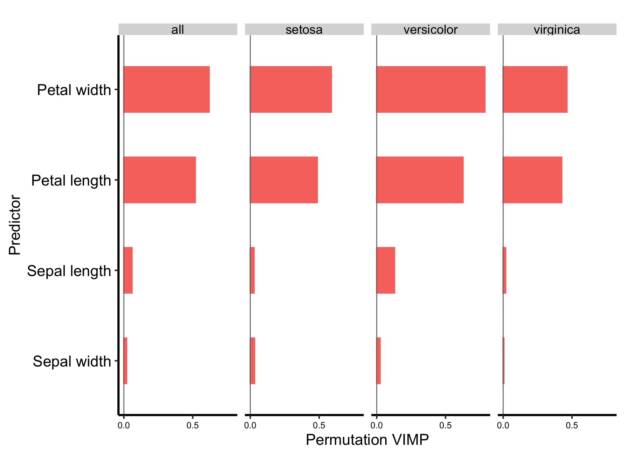
The size of the shift is the useful part. Petal length and petal width sit far above both sepal measurements in every run we have looked at, and that separation is what Figure 28.1 is for. The order within a close pair is not, at 300 trees. So read the grouping rather than the ranking. If an analysis needs the ranking, grow the forest until the ranking stops moving, and report how many trees that took.
28.5 Use display labels at plot time
Human-readable labels belong in the display, not in the model object. The current plot method uses labels. We confirm that applying those labels leaves the returned variables and their order unchanged.
# Free size: four facets (overall and one per class).vimp_plot +geom_hline(yintercept =0, color ="grey45", linewidth =0.35) +theme_hv_manuscript(base_size =12) +scale_y_continuous(breaks =function(x) pretty(x, n =3),expand =expansion(mult =c(0.05, 0.05)) ) +labs(x ="Predictor", y ="Permutation VIMP", fill ="VIMP > 0") +theme(axis.text.x =element_text(size =7))
Figure 28.1: Permutation VIMP overall and by iris class; display labels do not alter the stored predictor names. Teal bars mark predictors whose permutation worsened prediction (VIMP above zero), salmon-red bars those whose permutation improved it, and the gray horizontal line marks zero.
28.6 Read it
Start with the all facet for the global ranking, then inspect whether the class-specific facets tell the same story. Petal width and petal length carry most of the prediction in this fit. A predictor can rank differently by class because the forest may need it to distinguish one outcome more than another. The grey zero line separates positive from negative VIMP, and the axis range is set from the returned scores so neither negative values nor larger positive values are clipped.
The object contains point estimates, not confidence intervals. Small gaps near the bottom should not be treated as settled ranks. If the order matters to a manuscript conclusion, refit across seeds or use a resampling analysis and report that uncertainty separately.
28.7 Adapt it
For a survival or regression forest there is usually one outcome set. For a classification forest, inspect unique(vimp_dta$set) before deciding whether to report the global ranking or a class-specific one. gg_vimp(rf, nvar = 10) can reduce a long display, but keep the full ranking in a supplement when the cutoff affects interpretation.
28.8 Pitfalls
Reading sign as clinical direction. Positive VIMP means worse prediction after permutation, not that larger predictor values increase risk.
Calling VIMP an effect size. Scores depend on this forest, this outcome, this predictor set, and the prediction-error scale.
Ignoring correlated predictors. Shared information can be split or redistributed across variables.
Treating labels as data changes. Use labels in plot(). Keep the raw predictor names intact for downstream code and audit trails.
Claiming causality. VIMP describes predictive contribution. It does not identify an intervention effect.