The varPro chapter ranks and selects variables; this one asks the next question, how a selected variable moves the prediction. gg_partial_varpro() runs varPro::partialpro() on a fitted varpro object and tidies the result into marginal-effect curves: one panel per variable, the predicted response across that variable’s range with the rest of the design held as observed. Reach for it once selection has narrowed the field and you want to read the shape and direction of each survivor’s effect, not just its rank.
The y-axis is the part worth knowing in advance, because it depends on the outcome family and you can choose it. A scale argument sets what the curve plots: response units for regression, a probability or log-odds for classification, and survival probability, restricted mean survival time, or ensemble mortality for a survival fit. That choice is the difference between a figure a clinician reads at a glance and one only the modeller understands.
The default is scale = "auto", which reads the family off the fit: a classification forest resolves to probability, a survival forest to survival probability, and a regression forest to a generic scale. Generic still plots the response in its own units, but it labels the axis “Partial Effect” rather than naming the response, so a regression figure headed for a manuscript needs its own labs(y = ...). Auto needs the fitted object to read a family at all. Hand it precomputed partial-dependence data and no fit and it warns, then falls back to that same generic axis.
33.2 The data it needs
gg_partial_varpro() reads a fitted varpro object, so we build one of each family up front, reusing the datasets from the random-forest chapters: housing for regression, breast for classification, and pbc for survival.
Across all three the call is the same; only the scale (and, for survival, an optional time) changes. With wide data we pass nvars so partialpro only computes the top-ranked handful, because it is the expensive step, and on a survival fit it is expensive enough to matter.
nvars selects by importance, not by list position. The variables are reordered by their rank in varPro::get.topvars() first, and only then does nvars keep the top few, so nvars = 6 returns the six varPro ranked highest rather than the six that happened to come back first. The panels arrive sorted the same way, by importance rather than alphabetically, so the top-left panel is the strongest variable and you can read the grid in rank order.
33.3 Regression: the response scale
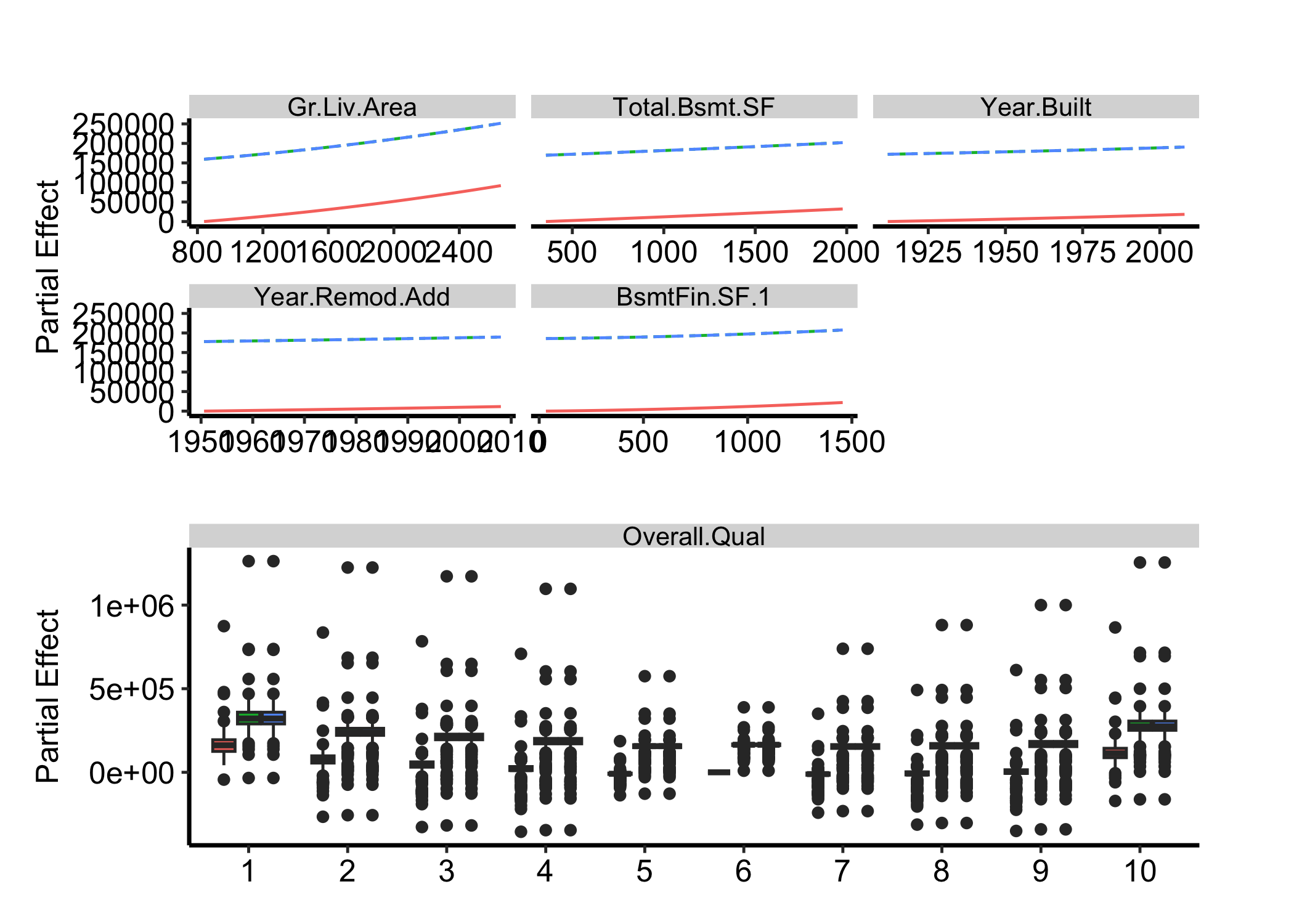
On a regression fit the y-axis is the response in its own units. Here that is SalePrice, so each curve reads as dollars of sale price across the predictor.
# Free size: one small-multiple panel per variable.plot(gg_partial_varpro(object = o_reg, nvars =6, method ="rnd")) &theme_hv_manuscript(base_size =12)
Figure 33.1: Partial-dependence curves for the top six predictors of the housing regression fit, plotted on the response scale in dollars of sale price. Each panel is one variable, with the black dashed line the parametric curve and the black solid line the nonparametric curve.
plot() returns a patchwork panel, so we theme it with &. A rising curve is a variable that pushes the prediction up over its range; a flat one is a variable the forest barely leans on once the others are fixed. The panels arrive in varPro importance order, so Gr.Liv.Area leading the grid is a statement about rank and not about the alphabet.
Note the y-axis label. The values are dollars, but a regression fit resolves to the generic scale and prints “Partial Effect”, which is the one place this chapter’s figures need a manual labs(y = "Sale price (USD)") before they go into a manuscript.
33.4 Classification: probability or log-odds
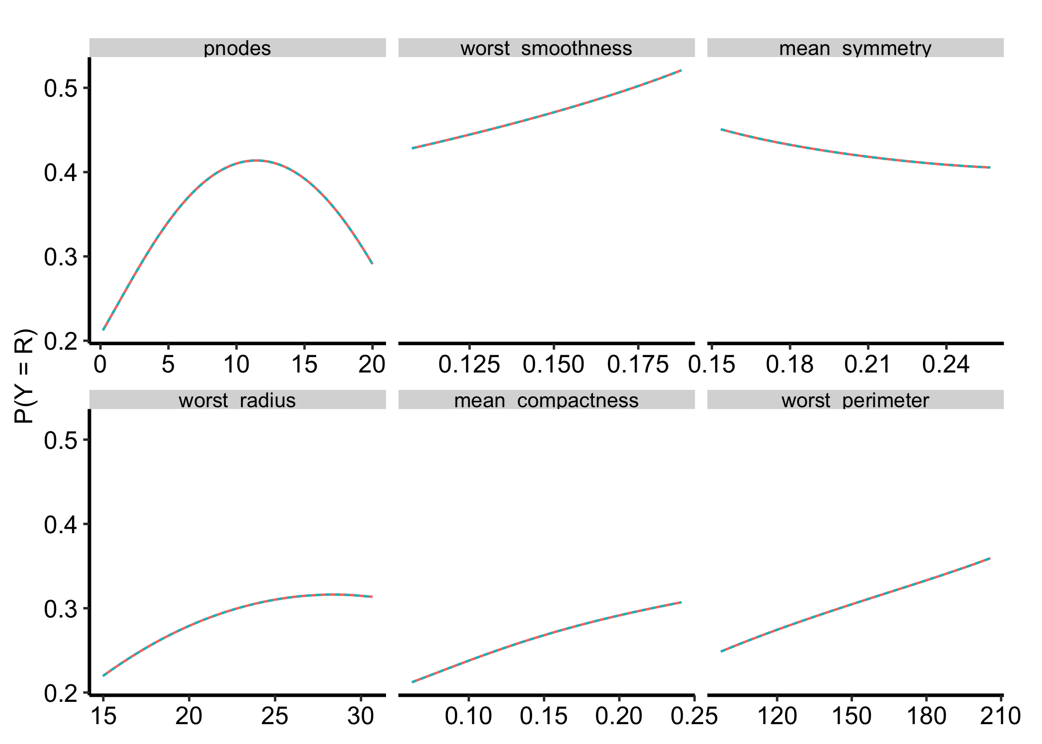
A classification fit defaults to probability, P(Y = the target class), bounded 0 to 1 and the scale a clinician expects.
# Free size: one small-multiple panel per variable.plot(gg_partial_varpro(object = o_cls, nvars =6, scale ="prob", method ="rnd")) &theme_hv_manuscript(base_size =12)
Figure 33.2: Partial dependence for the breast classification fit on the probability scale, bounded zero to one. Each panel is one variable, with the black dashed line the parametric curve and the black solid line the nonparametric curve.
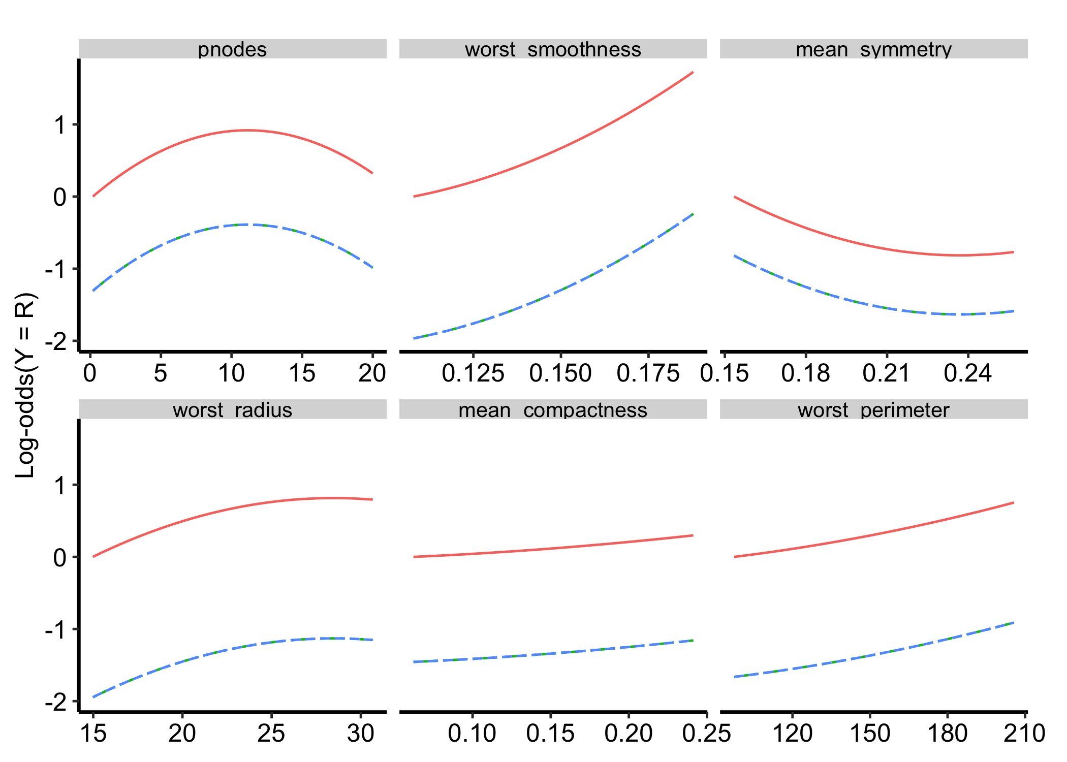
Setting scale = "logodds" plots the same effect on the log-odds scale, which is linear in the model’s own terms and is the only scale on which the causal (virtual-twins) contrast can be shown. The default draws only the parametric and nonparametric curves, so ask for causal by name in type. Use probability to communicate and log-odds to diagnose.
Figure 33.3: The same classification partial dependence on the log-odds scale, linear in the model’s own terms and the only scale showing the causal contrast. Each panel is one variable, with the black dotted line the parametric curve, the black dashed line the nonparametric curve, and the black solid line the causal contrast.
33.5 Survival: probability, RMST, or mortality
A survival fit gives you three readings of the same partial effect, and the choice is the whole point of the scale argument.
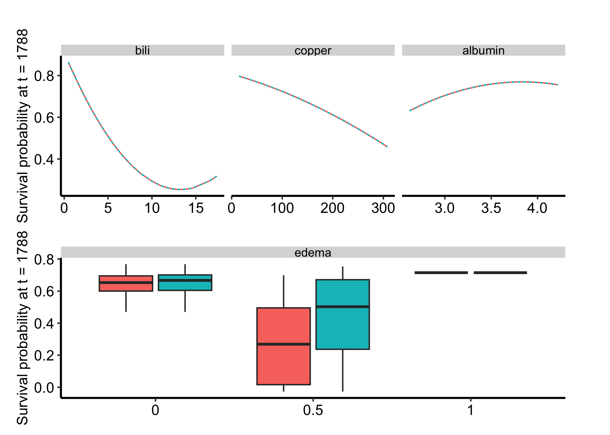
scale = "surv" (the default) plots survival probabilityS(tau | x), bounded 0 to 1 at a horizon tau. Leave time out and tau resolves to the median follow-up, printed on the axis label (here t = 1788), so you get a units-safe horizon without guessing.
# Free size: one small-multiple panel per variable.plot(gg_partial_varpro(object = o_surv, nvars =4, scale ="surv", method ="rnd")) &theme_hv_manuscript(base_size =12)
Figure 33.4: Partial dependence for the pbc survival fit on the survival-probability scale at the median follow-up horizon. Each panel is one variable, with the black dashed line the parametric curve and the black solid line the nonparametric curve.
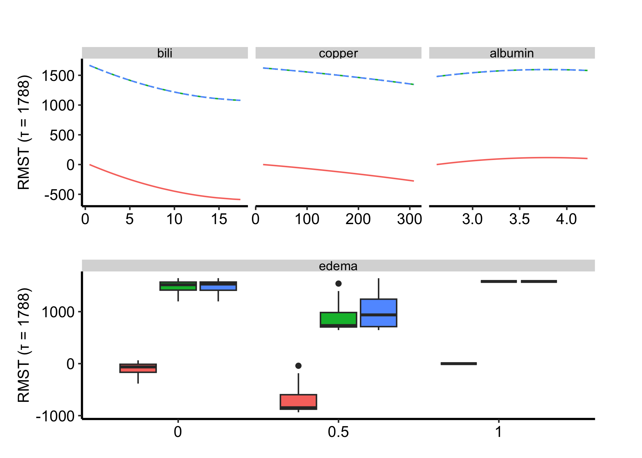
scale = "rmst" plots restricted mean survival time: the expected event-free time within the first tau days, read in the model’s own time units and higher-is-better. It answers “how much time does this variable buy?” rather than “what is the probability at tau.”
# Free size: one small-multiple panel per variable.plot(gg_partial_varpro(object = o_surv, nvars =4, scale ="rmst", method ="rnd")) &theme_hv_manuscript(base_size =12)
Figure 33.5: Partial dependence for the pbc survival fit on the restricted-mean-survival-time scale, read as event-free time within the horizon. Each panel is one variable, with the black dashed line the parametric curve and the black solid line the nonparametric curve.
The third option, scale = "mortality", is the unbounded ensemble-mortality score, where higher is worse, the opposite direction from the two bounded scales above. It is the right choice only when you are comparing against other random-forest mortality outputs; for a figure a reviewer reads, prefer surv or rmst.
33.6 How sure is the curve?
These curves come from one varPro fit, and a different sample of patients would give a different curve. Neither gg_partial_varpro() nor varPro::plot.partialpro() shows how different. plot.partialpro() does draw dotted lines at two standard errors, but they measure the spread across patients for this one fit, and they come out narrower still here because partialpro() returns every patient’s curve at the cohort-mean level. The Variable and partial dependence chapter sets out the reasoning. The recipe is the same here: refit on subsamples, recompute the curve, and rescale the spread by \(\sqrt{m/n}\)(Ishwaran and Lu 2019).
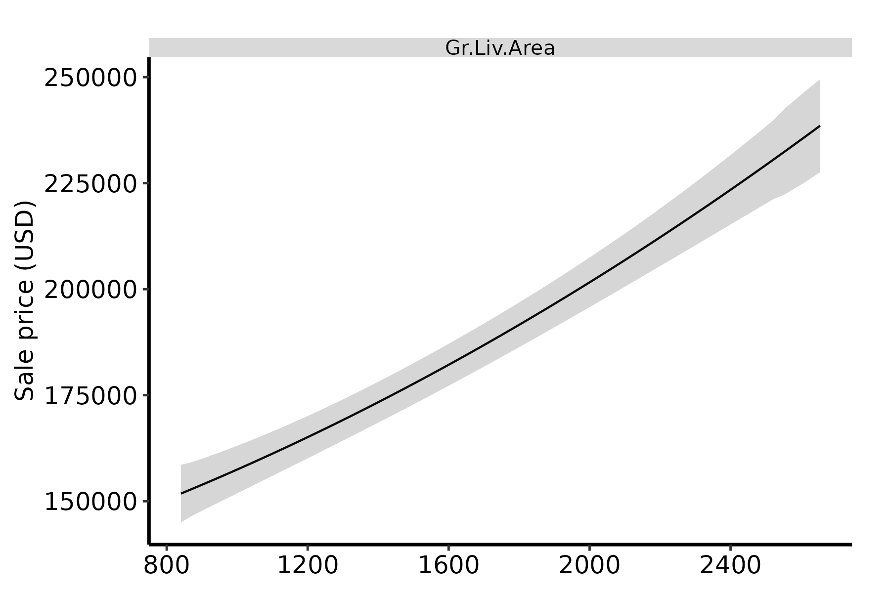
Two things change for varPro. Each refit reruns both varpro() and partialpro(), so it is slower than a forest refit. And partialpro() builds its grid from each refit’s own training data, with no argument to fix it, so we interpolate every refit’s curve onto the full fit’s grid with approx(). A refit whose data do not reach the extremes of the full grid leaves NA there, which sd(na.rm = TRUE) skips. We take one variable, the regression fit’s top-ranked Gr.Liv.Area, and subsample the rows varpro() kept after dropping incomplete cases. With n above 1,000, subsample()’s ratio shrinks to \(e^{-1}\sqrt{1000/n}\).
plot() returns a patchwork when a fit has categorical panels too, and + would then reach only the last of them. which = "continuous" asks for the single ggplot, which takes the ribbon like any other layer. type = "parametric" draws only the curve the band was built from, since the default adds the nonparametric curve, which the band says nothing about.
Figure 33.6: Partial dependence of sale price on above-ground living area for the housing regression fit, with a pointwise 95% band from 25 subsample refits. The solid black line is the parametric curve and the grey ribbon the pointwise 95% band.
Read it the way you read the forest band: a rise wider than the band survives resampling, and the band widens where few houses are that large. Budget for it. The full fit and one partial-dependence run take seconds each here, and the 25 refits in this chunk repeat both on 554 of the 2274 houses. The chunk is frozen after its first render, but on your own cohort, time one refit before choosing B.
33.7 Pitfalls
partialpro is the expensive step. It recomputes for every variable you ask for and, on a survival fit, for the whole time grid. Always cap it with nvars; under Quarto’s freeze the result is cached after the first render.
The y-axis depends on scale, and the default reads the family off the fit.scale = "auto" gives probability for classification and survival probability for survival, both of which name themselves on the axis. A regression fit resolves to the generic scale instead: the values are still response units, but the axis says “Partial Effect”, so add your own labs(y = ...) before anyone reads it as unitless. Without a fitted object auto cannot resolve at all; it warns and uses the same generic axis. State the scale in the caption either way, so a reader knows whether higher is better (surv, rmst) or worse (mortality).
nvars ranks before it slices. It keeps the top n by varPro importance, not the first n in the list it was handed, and the returned panels sort by importance rather than alphabetically. Raising nvars therefore extends the grid downward in rank; it does not reshuffle the panels you already had.
tau must be in the fit’s time units. For surv/rmst, a time beyond the largest event time truncates to the full restricted mean; omit time to let it default to the median follow-up.
The causal contrast only shows on logodds, and only when you ask for it. The default type leaves it out on every scale; on the bounded probability and survival scales it is hidden by design, so do not expect the virtual-twins estimate there.
Set method to "rnd" on every gg_partial_varpro() call. Its ... forwards straight to varPro::partialpro(), which grows its own isolation forest for the partial-dependence draws; leave method unset and that forest defaults to unsupv, handing randomForestSRC a zero-length yvar.wt pointer. Nothing breaks in practice, since the pointer is formed and never dereferenced, but the real fix belongs upstream. Set it anyway: every call in this chapter does, because these are the chunks readers copy.
Ishwaran, Hemant, and Min Lu. 2019. “Standard Errors and Confidence Intervals for Variable Importance in Random Forest Regression, Classification, and Survival.”Statistics in Medicine 38 (4): 558–82. https://doi.org/10.1002/sim.7803.