After the tree-count diagnostic is stable, we can ask what the forest predicts. For a survival forest the response is not one number. Each patient receives a survival function, the predicted probability of remaining event-free beyond each follow-up time.
Use gg_rfsrc() for model predictions and gg_survival() for the empirical Kaplan-Meier estimate. They answer related but different questions. One shows what the fitted forest predicts from all included covariates; the other summarizes the observed time-to-event experience without that model.
27.2 Fit a survival forest
The public veteran trial data contain follow-up time, death status, treatment arm, and baseline predictors. We use 300 trees to keep the recipe bounded. A production fit still needs its own tree-count stability check.
                         Sample size: 137
                    Number of deaths: 128
                     Number of trees: 300
           Forest terminal node size: 15
       Average no. of terminal nodes: 6.2533
No. of variables tried at each split: 3
              Total no. of variables: 6
       Resampling used to grow trees: swor
    Resample size used to grow trees: 87
                            Analysis: RSF
                              Family: surv
                      Splitting rule: logrank *random*
       Number of random split points: 10
                          (OOB) CRPS: 62.92693288
             (OOB) standardized CRPS: 0.06298992
   (OOB) Requested performance error: 0.30309059
27.3 Inspect OOB predicted survival
oob = TRUE is the constructor default for a training forest. Each patient’s curve is built from trees that did not use that patient to grow the tree.
          minimum           maximum monotone_subjects          subjects
                0                 1               137               137
The inspected object is long: obs_id identifies the patient, variable is the event-time grid, and value is predicted survival. Values stay between 0 and 1, and every subject’s curve is non-increasing.
plot(pred_oob, alpha =0.18) +theme_hv_manuscript(base_size =12) +labs(x ="Follow-up time (days)", y ="Predicted survival probability") +coord_cartesian(ylim =c(0, 1))
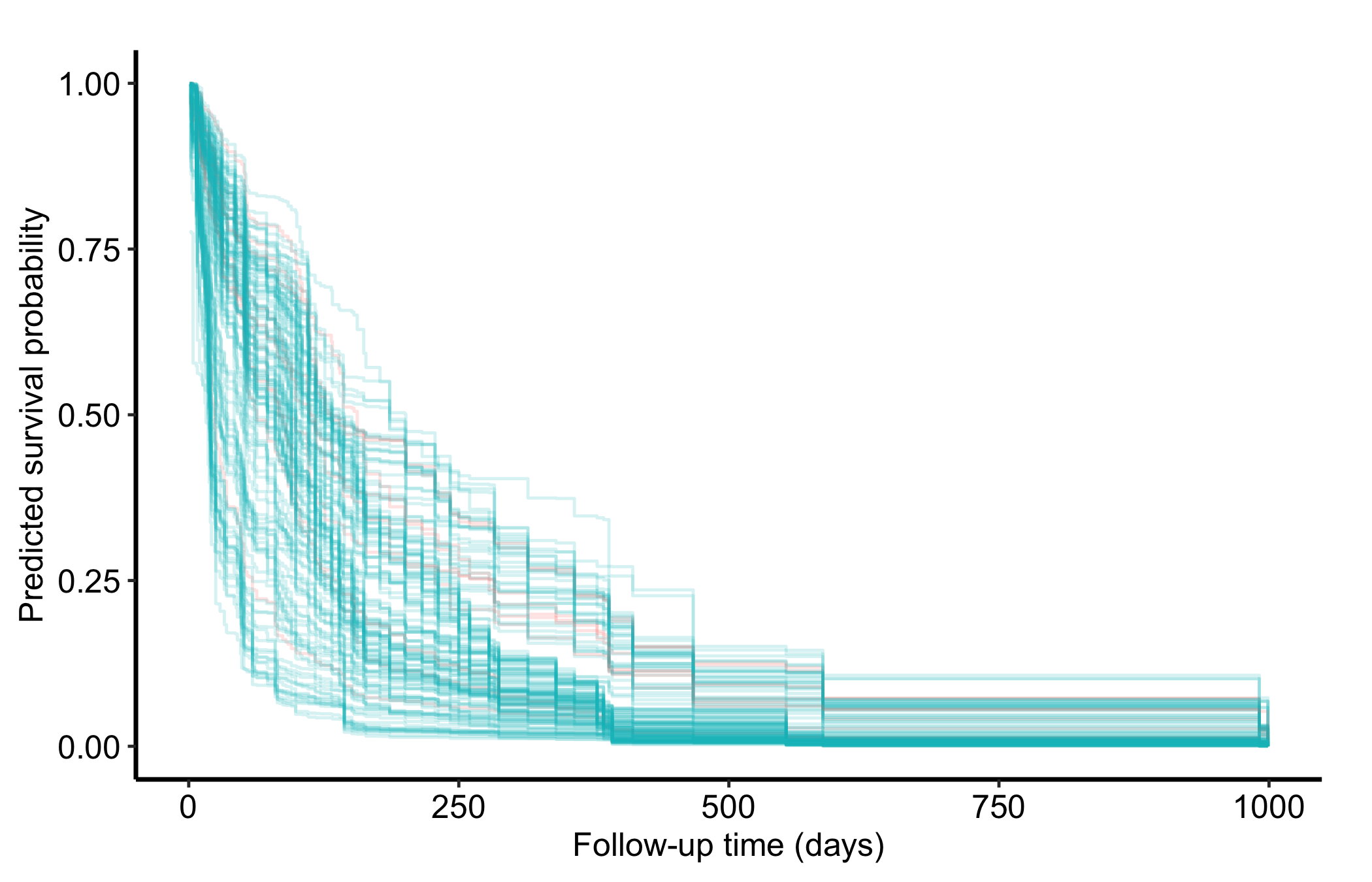
Figure 27.1: OOB predicted survival curves for the veteran cohort, one curve per patient. Each thin step line is one patient: salmon-red for patients censored and teal for patients who died.
Read the fan as predicted heterogeneity. Curves that fall earlier correspond to higher predicted risk. They are not observed patient trajectories, and the separation does not identify which covariate caused an outcome.
27.4 OOB versus in-sample predictions
Setting oob = FALSE uses the full forest, including trees that may have seen the patient during training. The two objects share the same scale, but the full-forest values are in-sample descriptions and can look more decisive.
                comparison survival_probability
1 Mean absolute difference           0.02643129
Use OOB predictions for an internal performance view. Use predictions from a separate validation cohort when the question is transportability.
27.5 Predicted and empirical survival by treatment arm
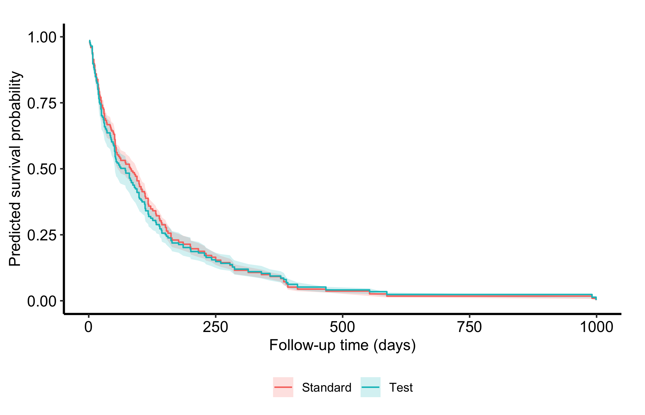
A grouped model display summarizes the patient-level predictions within each arm. With by = "trt", gg_rfsrc() resamples patients within each arm, computes the mean predicted survival at every time in each bootstrap sample, and returns the median of those bootstrap means with a pointwise 95% band. By default, the number of resamples for an arm equals the number of patients in that arm.
Thus the center line is not the survival curve for a median patient. The band describes resampling variation in the group mean conditional on this fitted forest; it does not display patient-to-patient heterogeneity and does not carry the full uncertainty from refitting the forest. The result remains descriptive of this fitted model, not an adjusted treatment effect or a hypothesis test.
pred_group <-gg_rfsrc(rf, by ="trt", conf.int =0.95)pred_group
  value     lower     upper    median      mean    group
1     1 0.9756614 0.9897106 0.9844840 0.9832853 Standard
2     2 0.9656496 0.9827440 0.9759916 0.9747951 Standard
3     3 0.9585212 0.9773103 0.9688330 0.9682215 Standard
4     4 0.9427702 0.9694694 0.9595628 0.9572675 Standard
plot(pred_group) +theme_hv_manuscript(base_size =12) +labs(x ="Follow-up time (days)", y ="Predicted survival probability",color ="Treatment arm", fill ="Treatment arm") +coord_cartesian(ylim =c(0, 1)) +theme(legend.position ="bottom")
Figure 27.2: Median bootstrap estimate of group-mean OOB predicted survival, with pointwise 95% bands within each veteran treatment arm. Step lines show the median estimate and shaded bands the 95% limits, salmon-red for the standard arm and teal for the test arm.
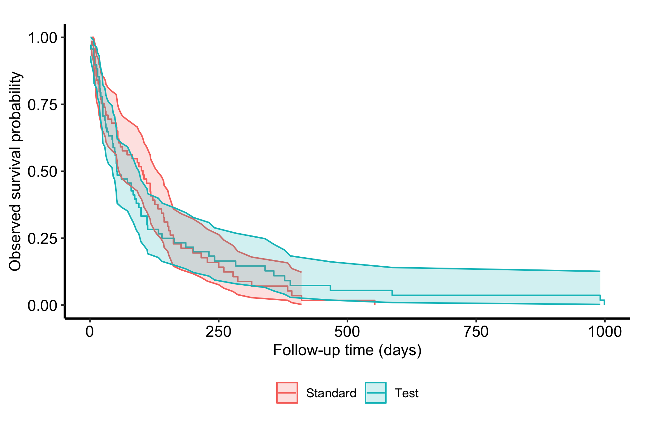
For the observed comparison, gg_survival() handles right-censoring directly. The censor argument names the event indicator here: status = 1 is death and status = 0 is censored.
km <-gg_survival(interval ="time",censor ="status",by ="trt",data = veteran)km
  time  n dead      surv   groups
1    3 69    1 0.9855072 Standard
2    4 68    1 0.9710145 Standard
3    7 67    1 0.9565217 Standard
4    8 66    2 0.9275362 Standard
plot(km) +theme_hv_manuscript(base_size =12) +labs(x ="Follow-up time (days)", y ="Observed survival probability",color ="Treatment arm", fill ="Treatment arm") +coord_cartesian(ylim =c(0, 1)) +theme(legend.position ="bottom")
Figure 27.3: Empirical Kaplan-Meier survival by veteran treatment arm. Step lines show the survival estimate and shaded bands the confidence limits, salmon-red for the standard arm and teal for the test arm.
The two displays should not be expected to coincide. The empirical curves use only treatment groups; the forest predictions use the full predictor set and then summarize those predictions by treatment.
27.6 Pitfalls
Calling predictions outcomes.pred_oob$value is a predicted survival probability. Death and censoring are stored separately in the observed data.
Ignoring the tail. Late estimates depend on fewer patients who remain under follow-up. Read apparent separation there cautiously.
Calling a grouped prediction causal. Averaging predictions by treatment does not control confounding, estimate a treatment effect, or test the arms.
Treating OOB as transport validation. OOB predictions are internal. A new CORR era, registry, or institution remains a new-data question.