23  Predict from a hazard model

23.1 When to use it

An additive hazard fit becomes clinically useful when it tells us how risk changes after the operation. Survival probability is the fraction of comparable patients expected to remain alive beyond a named time. Cumulative hazard is the event intensity accumulated through that time. Instantaneous hazard is the conditional event rate among patients still at risk, with units of deaths per patient-month here. It is not the observed number of deaths. The interval with the most deaths also depends on how many patients remain at risk and how wide the interval is, so it need not coincide with the peak hazard. In a multiphase model, the hazard curve can also show which early or constant process is contributing that rate.

This chapter refits every model it uses. You can copy it into a clean R session without first running the fitting chapter. The working pattern is the same throughout: fit the object, inspect it, predict on an explicit time grid, then plot and read the result.

23.2 Refit the models

The first fit is the reviewed intercept-only Weibull model for the public CABG cohort. Follow-up is recorded in months, so every rate we derive from its time grid is per patient-month.

data(cabgkul, package = "TemporalHazard")

fit <- hazard(
  time = cabgkul$int_dead,
  status = cabgkul$dead,
  theta = c(0.01, 1),
  dist = "weibull",
  fit = TRUE
)
summary(fit)
hazard model summary
  observations: 5880 
  predictors:   0 
  dist:         weibull 
  engine:       native-r-m2 
  converged:    TRUE 
  log-lik:      -3935.72 
  evaluations: fn=37, gr=9

Coefficients:
       estimate    std_error    z_stat       p_value
mu 0.0003613699 6.016407e-05  6.006407  1.896793e-09
nu 0.5944429760 2.346410e-02 25.334149 1.343733e-141
grid <- data.frame(
  time = seq(0.5, max(cabgkul$int_dead), length.out = 120)
)

23.3 Predict survival and cumulative hazard

With se.fit = TRUE, current predict.hazard() returns the estimate, delta-method standard error, and confidence limits. Survival limits stay between 0 and 1; cumulative-hazard limits stay positive. Both predictions refer to the same fitted curve on the same grid.

survival <- predict(
  fit, newdata = grid, type = "survival",
  se.fit = TRUE, level = 0.95
)
cumhaz <- predict(
  fit, newdata = grid, type = "cumulative_hazard",
  se.fit = TRUE, level = 0.95
)

pred <- data.frame(
  time = grid$time,
  survival,
  cumhazard = cumhaz$fit,
  cumhazard_lower = cumhaz$lower,
  cumhazard_upper = cumhaz$upper
)
head(pred)
      time       fit       se.fit     lower     upper   cumhazard
1 0.500000 0.9940617 0.0007198401 0.9924805 0.9953112 0.005955985
2 2.191828 0.9857643 0.0012801536 0.9830651 0.9880359 0.014338007
3 3.883656 0.9800565 0.0015667688 0.9768108 0.9828519 0.020145071
4 5.575484 0.9753334 0.0017694642 0.9717115 0.9784967 0.024975903
5 7.267313 0.9711860 0.0019296943 0.9672726 0.9746376 0.029237240
6 8.959141 0.9674316 0.0020643398 0.9632771 0.9711232 0.033110581
  cumhazard_lower cumhazard_upper
1     0.004699778     0.007547963
2     0.012036221     0.017079982
3     0.017296857     0.023462290
4     0.021737833     0.028696317
5     0.025689521     0.033274899
6     0.029301987     0.037414204
# Survival and cumulative hazard must describe the same fitted model.
max(abs(pred$fit - exp(-pred$cumhazard)))
[1] 0

The last value should be zero to numerical precision because \(S(t)=\exp\{-H(t)\}\). If it is not, first check that both predictions came from the same fit, profile, and time grid. That catches the common mistake of joining predictions made on different rows.

23.3.1 Survival against the empirical curve

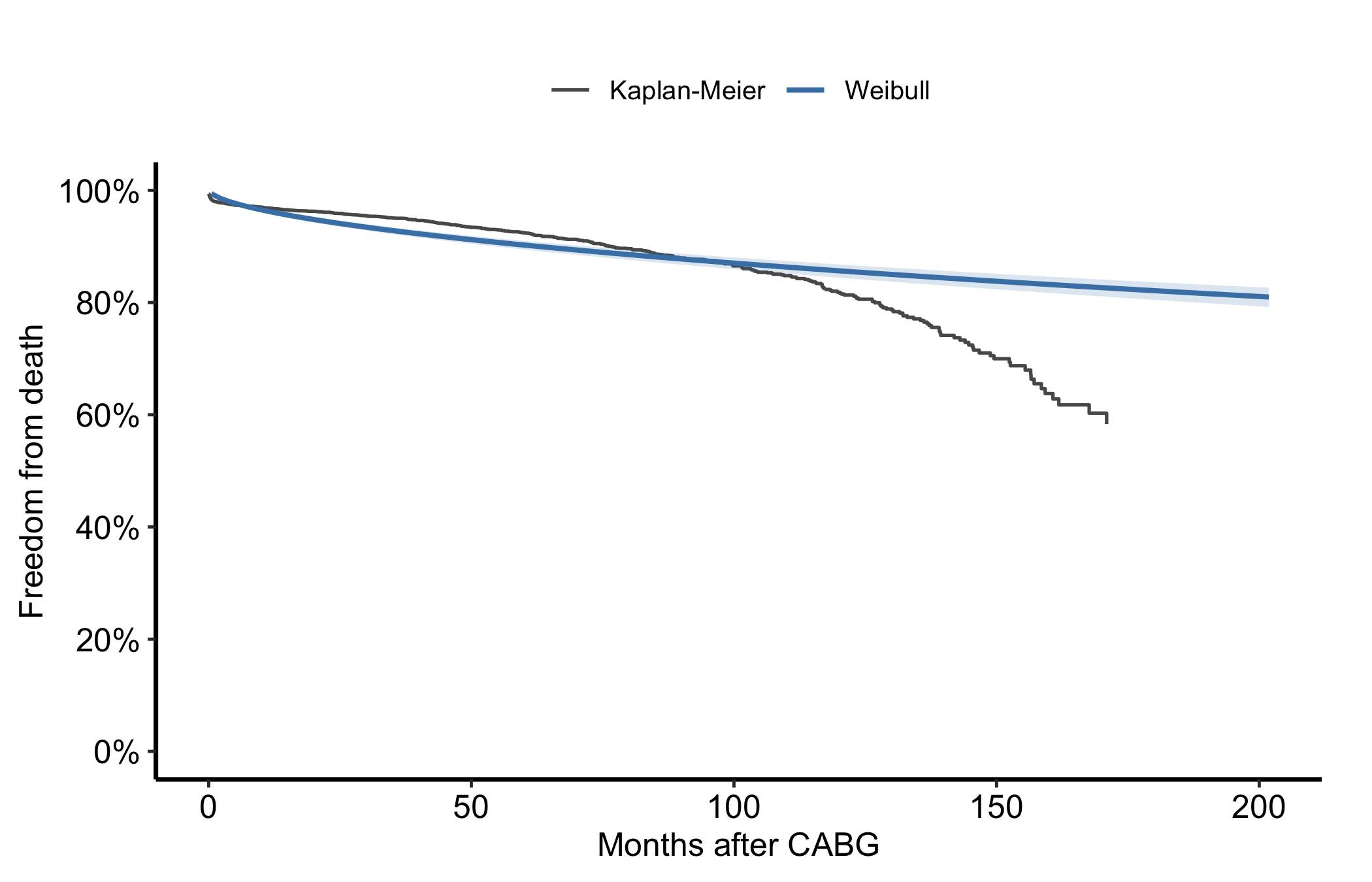
The smooth curve is a model result, so we judge it against the Kaplan-Meier estimate rather than letting it stand alone. The ribbon is uncertainty in the parametric curve; the step line is the empirical reference.

km <- hzr_kaplan(cabgkul$int_dead, cabgkul$dead)

ggplot() +
  geom_step(
    data = km,
    aes(time, survival * 100, colour = "Kaplan-Meier"),
    linewidth = 0.6
  ) +
  geom_ribbon(
    data = pred,
    aes(time, ymin = lower * 100, ymax = upper * 100),
    fill = "steelblue", alpha = 0.18
  ) +
  geom_line(
    data = pred,
    aes(time, fit * 100, colour = "Weibull"),
    linewidth = 0.9
  ) +
  scale_colour_manual(
    values = c("Kaplan-Meier" = "grey35", "Weibull" = "steelblue"),
    name = NULL
  ) +
  scale_y_continuous(limits = c(0, 100), breaks = seq(0, 100, 20),
                     labels = function(x) paste0(x, "%")) +
  labs(x = "Months after CABG", y = "Freedom from death") +
  theme_hv_manuscript() +
  theme(legend.position = "top")
Figure 23.1: Weibull survival with a 95% delta-method confidence band, overlaid on empirical Kaplan-Meier survival for the CABG cohort

The Weibull follows the broad decline but smooths over the changing early and late behavior in the empirical curve. A narrow band does not rescue a systematic shape mismatch; it only says the fitted parameters are estimated precisely under that Weibull model.

23.3.2 Accumulated event intensity

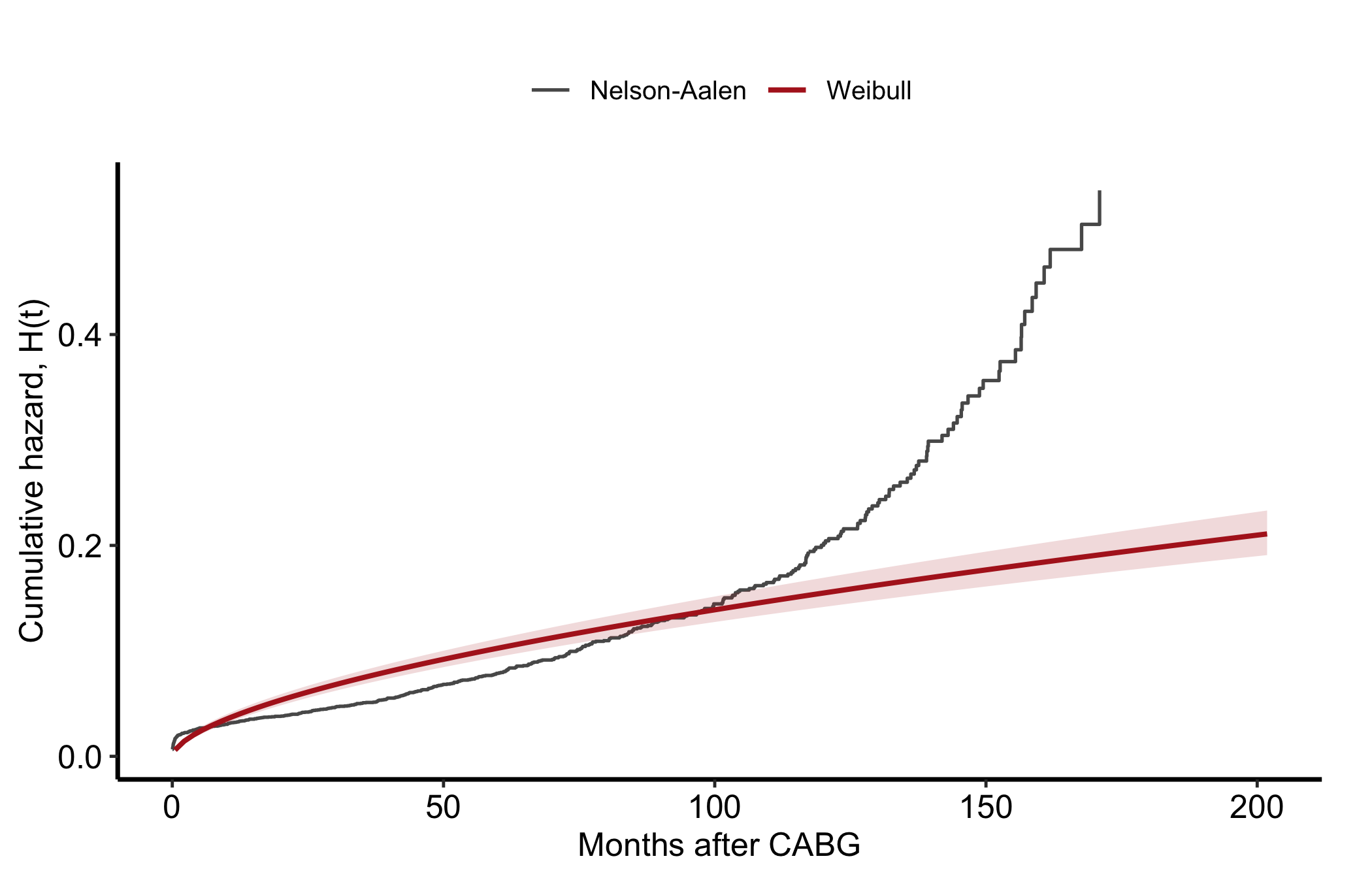
The Nelson-Aalen curve provides the corresponding empirical check for cumulative hazard. \(H(t)\) is dimensionless. Its slope, because time is in months, has units of events per patient-month.

na <- hzr_nelson(cabgkul$int_dead, cabgkul$dead)

ggplot() +
  geom_step(
    data = na,
    aes(time, cumhaz, colour = "Nelson-Aalen"),
    linewidth = 0.6
  ) +
  geom_ribbon(
    data = pred,
    aes(time, ymin = cumhazard_lower, ymax = cumhazard_upper),
    fill = "firebrick", alpha = 0.16
  ) +
  geom_line(
    data = pred,
    aes(time, cumhazard, colour = "Weibull"),
    linewidth = 0.9
  ) +
  scale_colour_manual(
    values = c("Nelson-Aalen" = "grey35", "Weibull" = "firebrick"),
    name = NULL
  ) +
  labs(x = "Months after CABG", y = "Cumulative hazard, H(t)") +
  theme_hv_manuscript() +
  theme(legend.position = "top")
Figure 23.2: Weibull cumulative hazard with a 95% delta-method confidence band, overlaid on the empirical Nelson-Aalen estimate

23.4 Predict an additive hazard directly

Now refit the reviewed AVC model. It has an early CDF phase and a constant phase, both on a monthly time scale. Current predict.hazard() supports direct instantaneous-hazard prediction for this multiphase model. We use that API; there is no need to approximate a derivative from cumulative-hazard values.

data(avc, package = "TemporalHazard")
avc <- na.omit(avc)

fit_multiphase <- hazard(
  survival::Surv(int_dead, dead) ~ 1,
  data = avc,
  dist = "multiphase",
  phases = list(
    early = hzr_phase(
      "cdf", t_half = 0.5, nu = 1, m = 1,
      fixed = "shapes"
    ),
    constant = hzr_phase("constant")
  ),
  fit = TRUE,
  control = list(n_starts = 3, maxit = 500)
)
summary(fit_multiphase)
Multiphase hazard model (2 phases)
  observations: 305 
  predictors:   0 
  dist:         multiphase 
  phase 1:      early - cdf (early risk)
  phase 2:      constant - constant (flat rate)
  engine:       native-r-m2 
  converged:    TRUE 
  log-lik:      -228.029 
  evaluations: fn=32, gr=10

Coefficients (internal scale):

  Phase: early (cdf)
               estimate std_error    z_stat     p_value
  log_mu     -1.4132735 0.1290435 -10.95192 6.50568e-28
  log_t_half -0.6931472        NA        NA          NA
  nu          1.0000000        NA        NA          NA
  m           1.0000000        NA        NA          NA

  Phase: constant (constant)
          estimate std_error    z_stat      p_value
  log_mu -7.609476 0.4495827 -16.92564 2.911483e-64
phase_grid <- data.frame(
  time = exp(seq(log(0.01), log(max(avc$int_dead)), length.out = 240))
)

total_hazard <- predict(
  fit_multiphase, newdata = phase_grid, type = "hazard",
  se.fit = TRUE, level = 0.95
)
total_cumhaz <- predict(
  fit_multiphase, newdata = phase_grid, type = "cumulative_hazard",
  se.fit = TRUE, level = 0.95
)
head(total_hazard)
        fit     se.fit     lower     upper
1 0.4682877 0.06034904 0.3637617 0.6028490
2 0.4675253 0.06025065 0.3631696 0.6018672
3 0.4667330 0.06014842 0.3625544 0.6008470
4 0.4659100 0.06004222 0.3619153 0.5997871
5 0.4650550 0.05993189 0.3612514 0.5986860
6 0.4641670 0.05981729 0.3605618 0.5975424

The instantaneous hazard and its confidence limits have units of deaths per patient-month. The cumulative hazard is dimensionless. Keep those labels separate even though the two quantities come from the same fit.

23.5 Rebuild and verify the phase contributions

hzr_phase_hazard() and hzr_phase_cumhaz() return unit-scale temporal shapes. Multiply each by its fitted scale, exp(log_mu), to recover that phase’s contribution. The helper signatures mirror the phase specification: the early CDF uses t_half, nu, and m; the constant phase needs only its type.

theta <- coef(fit_multiphase)
early_scale <- exp(theta["early.log_mu"])
constant_scale <- exp(theta["constant.log_mu"])

early_hazard <- early_scale * hzr_phase_hazard(
  phase_grid$time, t_half = 0.5, nu = 1, m = 1, type = "cdf"
)
constant_hazard <- constant_scale * hzr_phase_hazard(
  phase_grid$time, type = "constant"
)

early_cumhaz <- early_scale * hzr_phase_cumhaz(
  phase_grid$time, t_half = 0.5, nu = 1, m = 1, type = "cdf"
)
constant_cumhaz <- constant_scale * hzr_phase_cumhaz(
  phase_grid$time, type = "constant"
)

additivity_check <- data.frame(
  quantity = c("Instantaneous hazard", "Cumulative hazard"),
  maximum_absolute_difference = c(
    max(abs(total_hazard$fit - early_hazard - constant_hazard)),
    max(abs(total_cumhaz$fit - early_cumhaz - constant_cumhaz))
  )
)
additivity_check
              quantity maximum_absolute_difference
1 Instantaneous hazard                1.246832e-17
2    Cumulative hazard                2.775558e-17
stopifnot(
  additivity_check$maximum_absolute_difference[1] < 1e-12,
  additivity_check$maximum_absolute_difference[2] < 1e-12
)

Both differences should be at floating-point noise. If they are not, check the phase type, fixed shape values, time units, and fitted scale before plotting. The total must equal the phase sum at every time.

hazard_df <- rbind(
  data.frame(time = phase_grid$time, hazard = total_hazard$fit,
             component = "Total"),
  data.frame(time = phase_grid$time, hazard = early_hazard,
             component = "Early"),
  data.frame(time = phase_grid$time, hazard = constant_hazard,
             component = "Constant")
)
hazard_df$component <- factor(
  hazard_df$component, levels = c("Total", "Early", "Constant")
)

ggplot(hazard_df, aes(time, hazard, colour = component,
                      linetype = component)) +
  geom_ribbon(
    data = data.frame(phase_grid, total_hazard),
    aes(time, ymin = lower, ymax = upper),
    inherit.aes = FALSE, fill = "grey35", alpha = 0.14
  ) +
  geom_line(aes(linewidth = component)) +
  scale_colour_manual(
    values = c("Total" = "grey20", "Early" = "firebrick",
               "Constant" = "steelblue"),
    name = NULL
  ) +
  scale_linetype_manual(
    values = c("Total" = "solid", "Early" = "dashed",
               "Constant" = "dashed"),
    name = NULL
  ) +
  scale_linewidth_manual(
    values = c("Total" = 1, "Early" = 0.75, "Constant" = 0.75),
    guide = "none"
  ) +
  scale_x_log10(
    breaks = c(0.01, 0.1, 0.5, 1, 5, 20, 100),
    labels = c("0.01", "0.1", "0.5", "1", "5", "20", "100")
  ) +
  scale_y_log10(
    breaks = c(0.0005, 0.001, 0.005, 0.01, 0.05, 0.1, 0.5),
    labels = c("0.0005", "0.001", "0.005", "0.01", "0.05", "0.1", "0.5")
  ) +
  labs(x = "Months after AVC repair (log scale)",
       y = "Deaths per patient-month (log scale)") +
  theme_hv_manuscript() +
  theme(legend.position = "top")
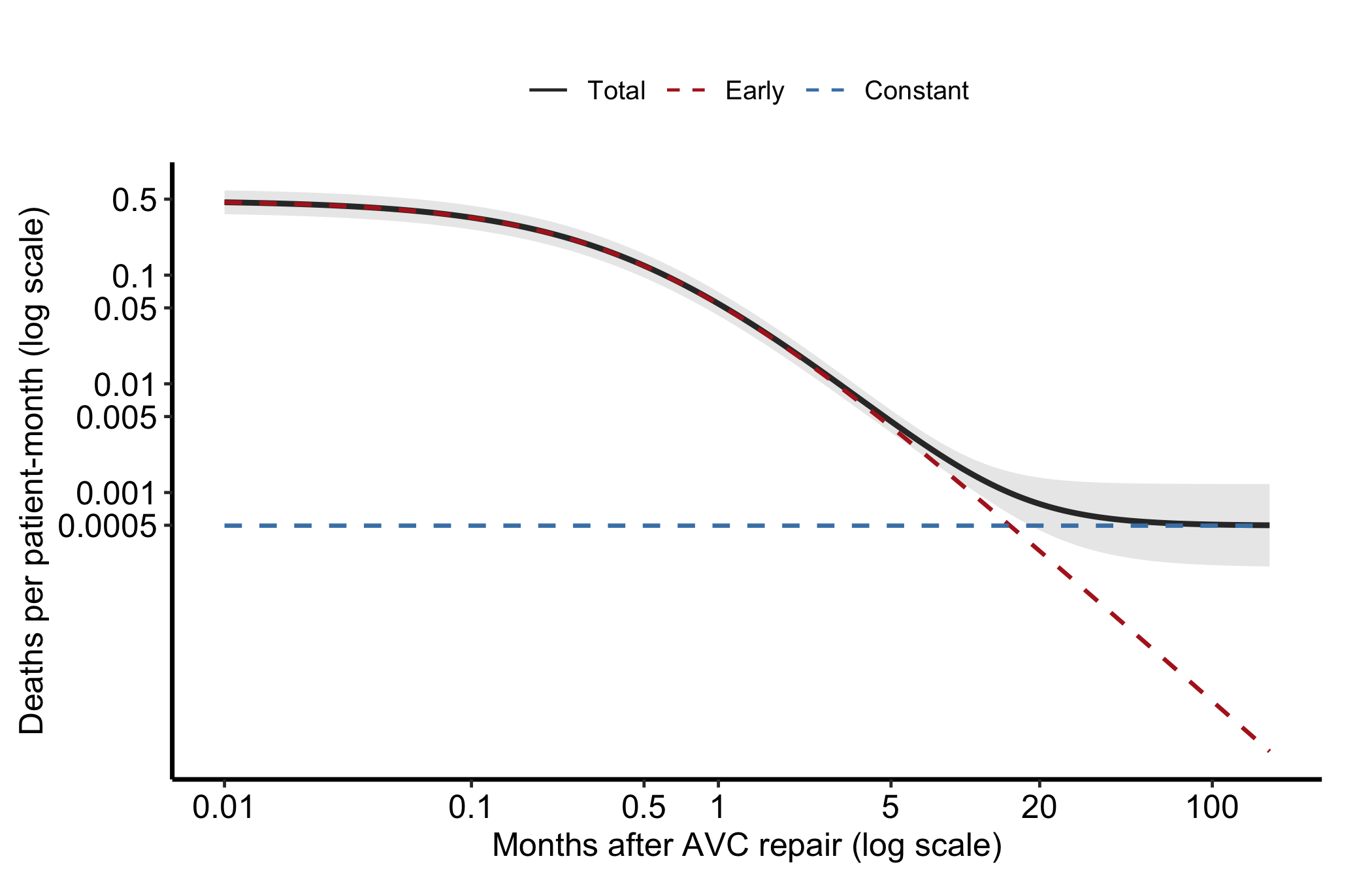
Figure 23.3: Fitted AVC hazard per patient-month: the total with its 95% confidence band and the additive early and constant contributions

The log scales keep the first postoperative days and the low constant rate visible on one panel. The early contribution dominates immediately after repair and then falls. The constant contribution is small and flat. Their sum is the solid total curve. If the phase order is clinically implausible, do not relabel it into a better story. Return to the empirical curve and the phase specification.

cumhaz_df <- rbind(
  data.frame(time = phase_grid$time, cumhaz = total_cumhaz$fit,
             component = "Total"),
  data.frame(time = phase_grid$time, cumhaz = early_cumhaz,
             component = "Early"),
  data.frame(time = phase_grid$time, cumhaz = constant_cumhaz,
             component = "Constant")
)
cumhaz_df$component <- factor(
  cumhaz_df$component, levels = c("Total", "Early", "Constant")
)

ggplot(cumhaz_df, aes(time, cumhaz, colour = component,
                      linetype = component)) +
  geom_ribbon(
    data = data.frame(phase_grid, total_cumhaz),
    aes(time, ymin = lower, ymax = upper),
    inherit.aes = FALSE, fill = "grey35", alpha = 0.14
  ) +
  geom_line(aes(linewidth = component)) +
  scale_colour_manual(
    values = c("Total" = "grey20", "Early" = "firebrick",
               "Constant" = "steelblue"),
    name = NULL
  ) +
  scale_linetype_manual(
    values = c("Total" = "solid", "Early" = "dashed",
               "Constant" = "dashed"),
    name = NULL
  ) +
  scale_linewidth_manual(
    values = c("Total" = 1, "Early" = 0.75, "Constant" = 0.75),
    guide = "none"
  ) +
  labs(x = "Months after AVC repair", y = "Cumulative hazard, H(t)") +
  theme_hv_manuscript() +
  theme(legend.position = "top")
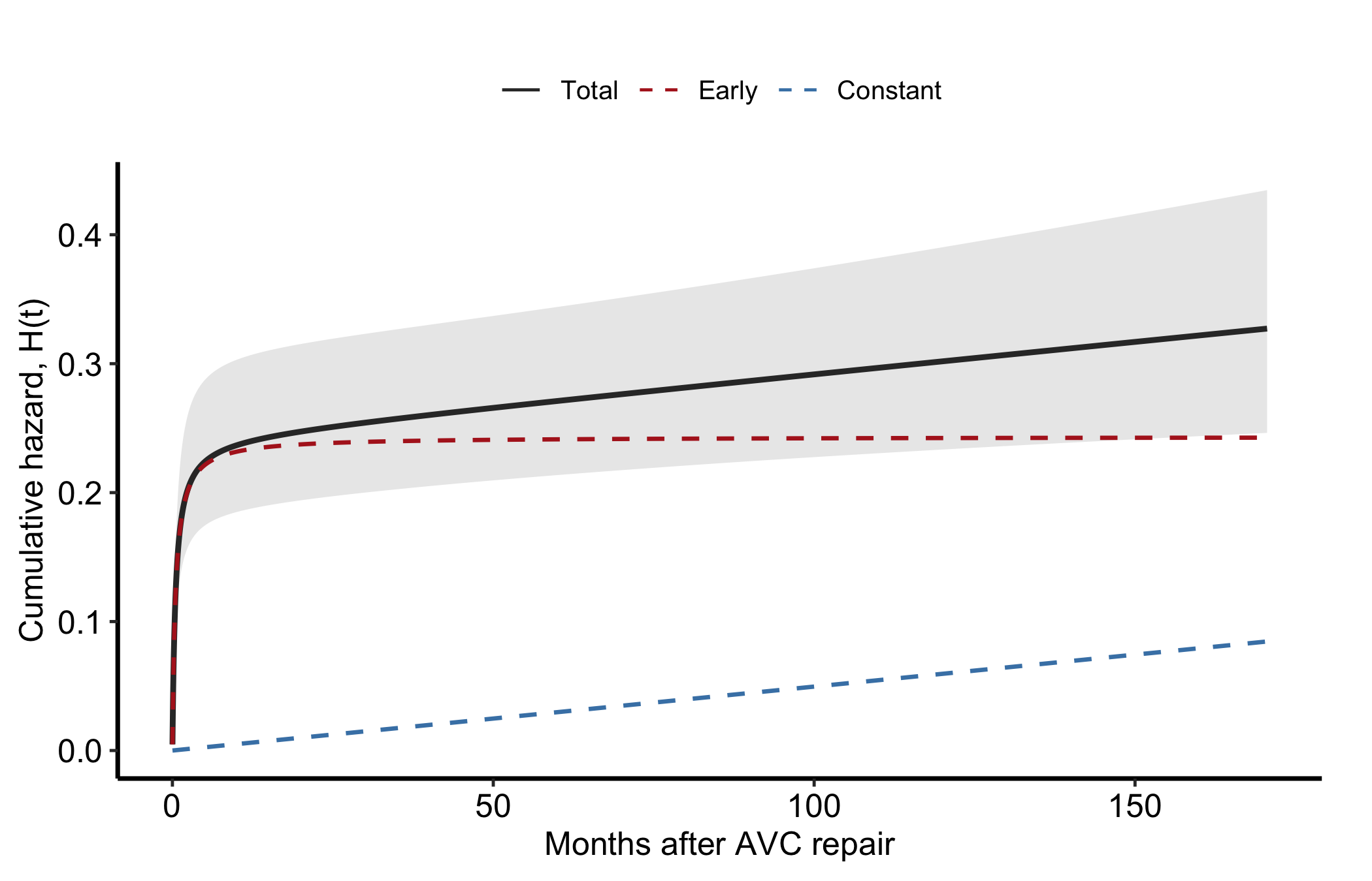
Figure 23.4: Fitted AVC cumulative hazard: the total with its 95% confidence band and the additive early and constant contributions

The early cumulative contribution rises quickly and then approaches a plateau. The constant contribution keeps accumulating linearly, even though its instantaneous rate is low. Thus a phase can look small on the hazard panel and still matter over long follow-up. Read the two panels together.