dta_trends <- sample_trends_data(n = 600, seed = 42)
p_base <- plot(hv_trends(dta_trends))7 Color templates for consistency
hvtiPlotR plots carry no colour scale by default. ggplot2’s (Wickham et al. 2026) scale_colour_* controls line and point colours; scale_fill_* controls filled areas (ribbons, bars). Both take the same name (legend title) and guide (legend display) arguments. Set them together so the two scales stay in sync.
7.1 When to use it
Colour is the fastest way to separate groups on a figure, and the easiest to overuse. Reach for a manual colour scale when the groups have a convention you want to honour (a brand colour, red for the high-risk arm) or when you have one series and simply want it off the default grey. Reach for a ColorBrewer palette when the groups are arbitrary and you want a set of hues that stay distinct in print and for colour-blind readers. And reach for legend suppression whenever the figure already names its groups some other way, since a colour that needs no key earns back panel space.
The guiding question is what the colour is for. If it carries information, the distinct group it marks, it has to survive a black-and-white printer and a colour-blind reader, which is where palette choice and a second visual channel come in. If it is decoration, keep it to one or two restrained hues. We use a grouped trends plot below so the colour mapping is visible across levels.
7.2 Manual colours
Use scale_colour_manual() / scale_fill_manual() to assign specific brand or convention colours to known levels. Here a single-stratum KM curve is set to one colour.
dta_km <- sample_survival_data(n = 500, seed = 42)
km     <- hv_survival(dta_km)

plot(km) +
  scale_color_manual(values = c(All = "steelblue"), guide = "none") +
  scale_fill_manual(values  = c(All = "steelblue"), guide = "none") +
  scale_y_continuous(breaks = seq(0, 100, 20),
                     labels = function(x) paste0(x, "%")) +
  scale_x_continuous(breaks = seq(0, 20, 5)) +
  coord_cartesian(xlim = c(0, 20), ylim = c(0, 100)) +
  labs(x = "Years after Operation", y = "Freedom from Death (%)") +
  theme_hv_manuscript()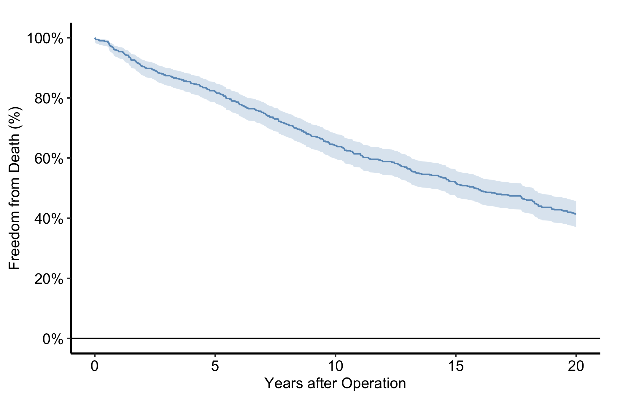
7.3 ColorBrewer palettes
scale_colour_brewer() applies a perceptually uniform, print-safe palette — which matters when figures go to black-and-white PDF. Use palette = "Set1" for categorical data, "RdYlGn" for diverging, "Blues" for sequential.
p_base +
  scale_colour_brewer(palette = "Set1", name = "Group") +
  scale_shape_manual(
    values = c("Group I" = 15, "Group II" = 19,
               "Group III" = 17, "Group IV" = 18),
    name = "Group"
  ) +
  labs(x = "Surgery Year", y = "Outcome") +
  theme_hv_manuscript()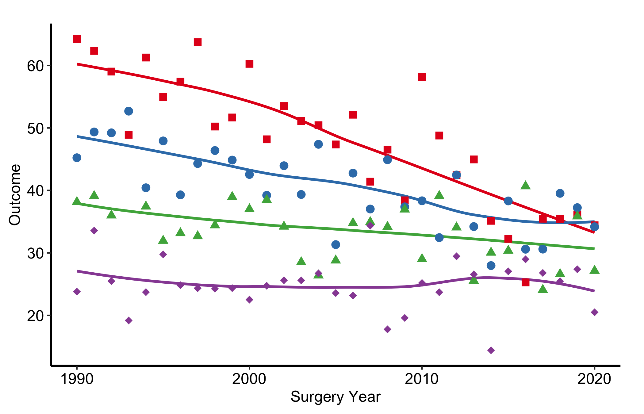
7.4 Suppressing legends
Pass guide = "none" to any scale and that aesthetic drops out of the legend. Do this when axis labels or an annotation already name the group, so a redundant legend does not eat panel space.
p_base +
  scale_colour_brewer(palette = "Dark2", guide = "none") +
  scale_shape_manual(
    values = c("Group I" = 15, "Group II" = 19,
               "Group III" = 17, "Group IV" = 18),
    guide = "none"
  ) +
  labs(x = "Surgery Year", y = "Outcome") +
  theme_hv_manuscript()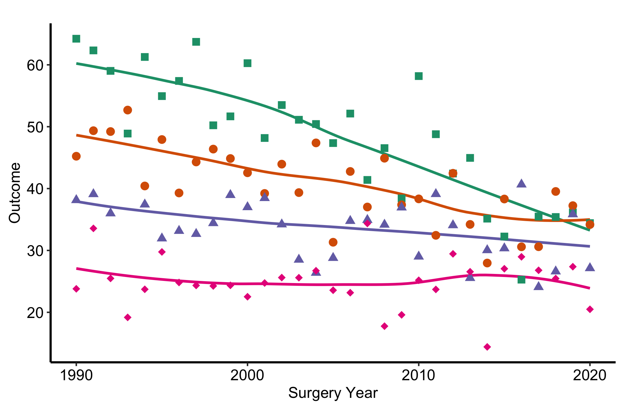
Notice that Figure 7.3 pairs colour with a distinct point shape per group. That redundancy is deliberate, and it is the heart of the first pitfall below.
7.5 Pitfalls
- Colour as the only channel. If the only thing separating two groups is their hue, the figure fails for a sizeable fraction of readers (red-green colour blindness alone affects roughly one man in twelve) and for anyone who prints it in greyscale, where two mid-tone colours collapse to the same grey. The fix is cheap: give each group a second channel as well, a point shape or a line type, so the distinction survives even when the colour does not. The recipes here map
scale_shape_manual()alongside the colour scale for exactly this reason. A quick check is to convert the figure to greyscale and confirm you can still tell the groups apart. - Too many hues. A palette with eight saturated colours does not help a reader; it asks them to memorise a legend and hunt for matches. Past about four or five groups, distinct colours stop being distinct and the figure turns to confetti. When you have many series, consider showing fewer at once, faceting into small panels, or muting the background series in grey and colouring only the one or two you are making a point about. Restraint reads as confidence.