28 ROC and Brier performance – HVTI ggplot graphics recipes

28.1 When to use it

A classification forest does not just label each patient, it returns a probability for each class, and a probability is only useful if you can say how trustworthy it is. Reach for these plots whenever you need to report how well a classification forest performs: whether it can tell recurrence from non-recurrence, how it compares against another model, or whether the predicted probabilities are calibrated well enough to act on. They are the performance half of any classification result, the figures a reviewer looks for right after the model description.

We judge a probabilistic classifier the same way we judge any other:

The ROC curve traces the trade-off between the true-positive rate (sensitivity, the share of true events you catch) and the false-positive rate (1 minus specificity, the share of non-events you wrongly flag) as the decision threshold sweeps from 0 to 1. The area under the curve (AUC) boils that whole curve down to one number: 0.5 is a coin flip, 1.0 is perfect separation.
The Brier score measures calibration, the mean squared difference between predicted probabilities and observed outcomes. Lower is better.

Both come from ggRandomForests (Ehrlinger 2026), and a useful detail comes for free: these are computed out-of-bag (from patients each tree never saw during fitting), so they are honest estimates that need no separate test set.

28.2 The data it needs

ROC reads from a fitted classification forest, one whose outcome is a factor so the forest predicts class probabilities. We use the Pima Indians diabetes data from mlbench (Leisch and Dimitriadou 2026) — 768 patients with eight clinical measurements and a two-level diabetes outcome — a forest that discriminates well enough to draw a ROC curve worth reading.

data(PimaIndiansDiabetes, package = "mlbench")
levels(PimaIndiansDiabetes$diabetes)

[1] "neg" "pos"

rf <- rfsrc(diabetes ~ ., data = PimaIndiansDiabetes, ntree = 100)
rf$family

[1] "class"

The family field confirms a classification forest, and the levels are neg (no diabetes) and pos (diabetes). The clinically interesting event is a positive diagnosis, so that is the class we will treat as positive.

28.3 Build it

gg_roc() builds the out-of-bag ROC curve for one outcome. The which_outcome argument names the class to treat as positive, and the important thing is that it takes a numeric index, not the level name: 2 selects the second level, pos. Pass the string "pos" and the call errors with “subscript out of bounds”.

plot(gg_roc(rf, which_outcome = 2)) + theme_hv_manuscript()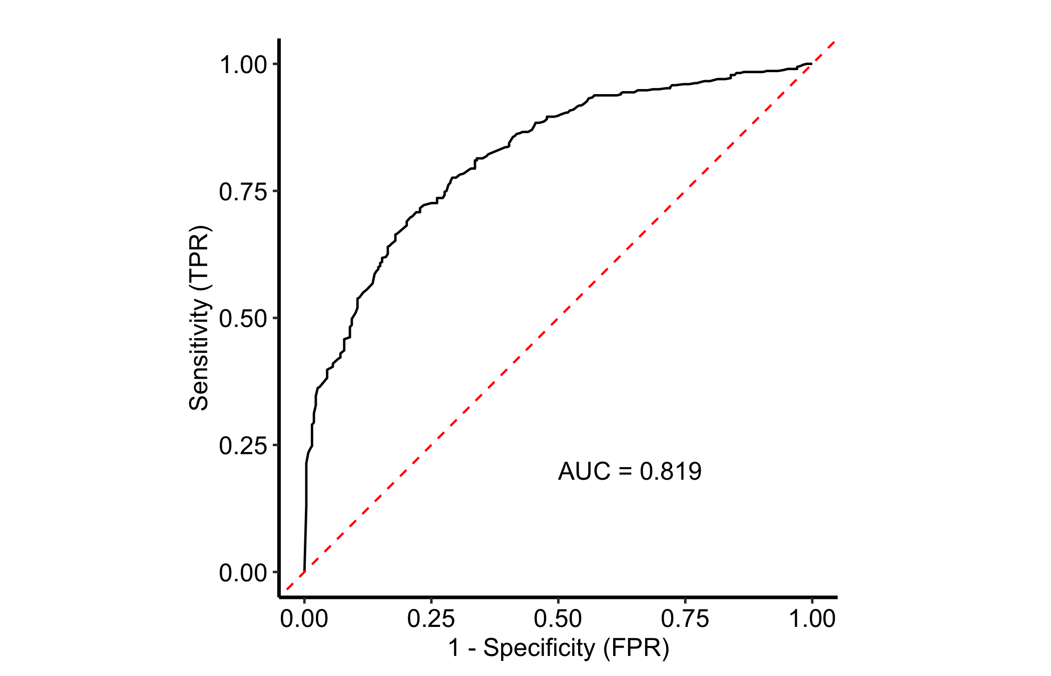

Figure 28.1: Out-of-bag ROC curve for the Pima diabetes classification forest, treating a positive diagnosis as the event, with the AUC printed on the panel

The curve bows toward the top-left corner. The further it pulls away from the diagonal (the line a random classifier would trace), the better the forest separates diabetic from non-diabetic patients, and the AUC printed on the panel quantifies that gap.

28.4 Read it

Distance from the diagonal is discrimination. A curve hugging the top-left corner means the forest ranks events above non-events almost every time; a curve sagging toward the 45-degree line means it is barely better than guessing. The AUC is that distance as a single number, easy to compare across models.
AUC ranks, Brier calibrates. AUC tells you whether the ranking is right, whether events get higher predicted probabilities than non-events. It says nothing about whether a predicted 0.8 actually happens 80% of the time. That is calibration, and it is what the Brier score checks. A forest can rank well (high AUC) yet be poorly calibrated, so read both.
Read per-class curves against each other. In the multi-class plot (Figure 28.2), the class whose curve sags closest to the diagonal is the one the forest finds hardest to separate from the rest. That is usually the more informative finding than the overall headline number.

28.5 Variations

28.5.1 Multi-class ROC

With more than two classes you draw one curve per class, each class treated as positive in turn against all the others (one-vs-rest). The per_class = TRUE flag does this in a single call. We illustrate on iris, where the three species give three curves.

rf_iris <- rfsrc(Species ~ ., data = iris, ntree = 100)
plot(gg_roc(rf_iris, which_outcome = 1, per_class = TRUE)) +
  theme_hv_manuscript()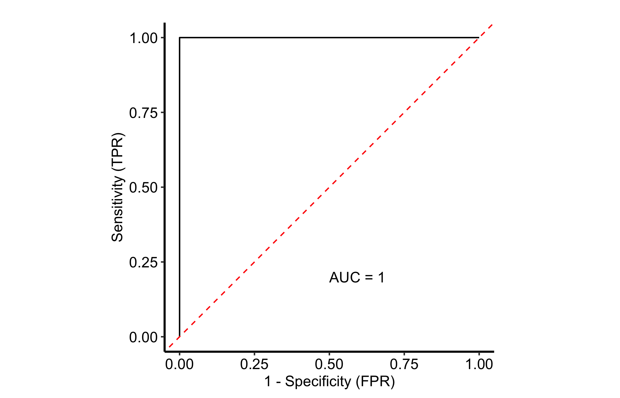

Figure 28.2: One-vs-rest ROC curves for the three iris species, one curve per class treated as positive in turn

Each coloured curve is one species-versus-rest classifier. The well-separated species hug the top-left corner; any class whose curve sags toward the diagonal is the one the forest struggles to tell apart from the others.

28.5.2 Brier score (on a survival forest)

The Brier score is a calibration measure, but in ggRandomForests gg_brier() only supports right-censored survival forests. It errors on a classification forest, so we cannot run it on the Pima diabetes model above; instead we refit pbc as a survival forest and plot the integrated Brier score over follow-up time, the survival analogue of the calibration check we want for classification.

data(pbc, package = "randomForestSRC")
rf_surv <- rfsrc(Surv(days, status) ~ ., data = pbc, ntree = 100)
plot(gg_brier(rf_surv)) + theme_hv_manuscript()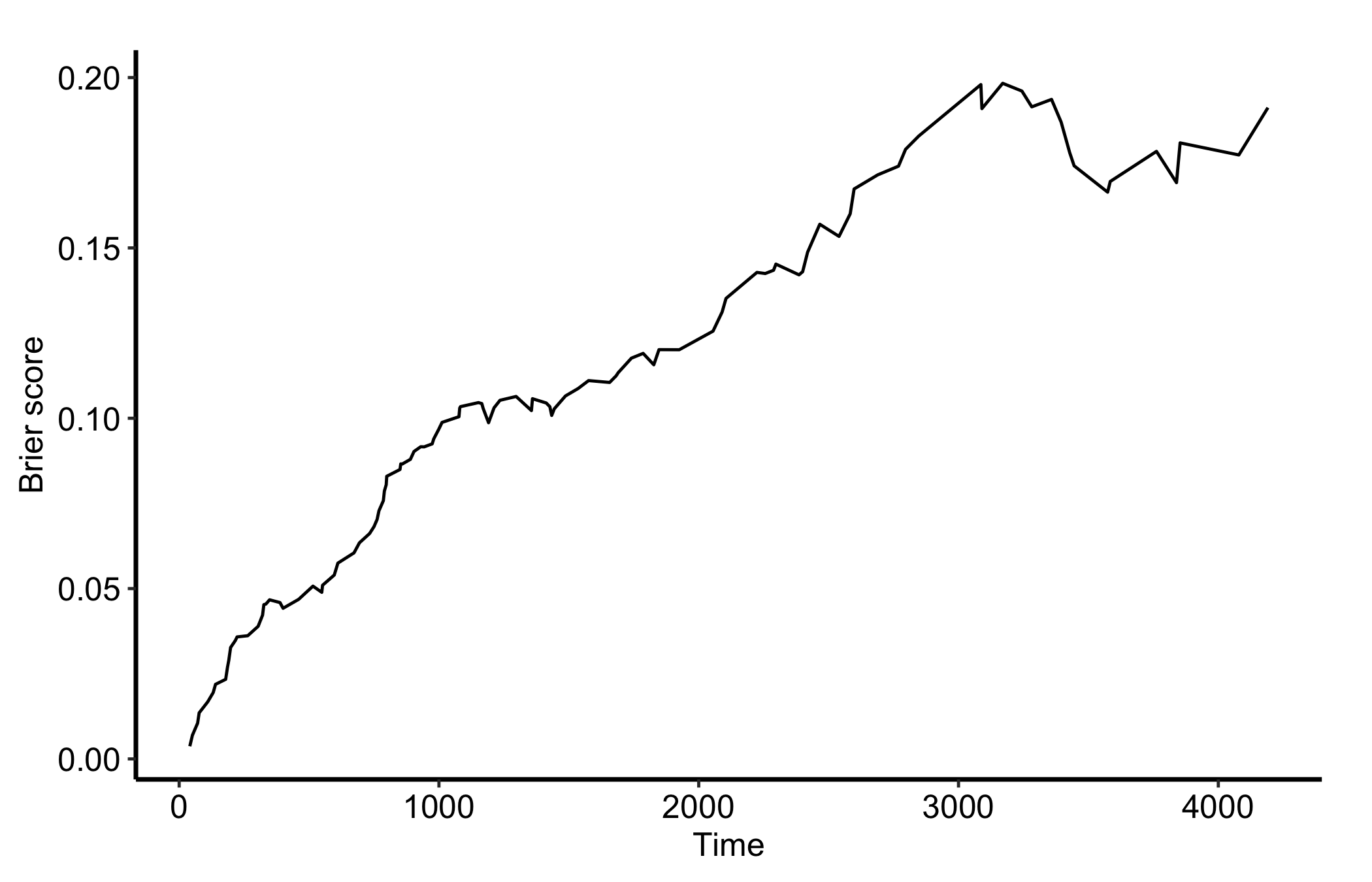

Figure 28.3: Integrated Brier score over follow-up time for a pbc survival forest, where lower curves mean better-calibrated predictions

Lower curves mean better-calibrated survival predictions across time. Read it alongside the error curve and AUC: discrimination (ROC and AUC) tells you whether the ranking is right, while the Brier score tells you whether the predicted probabilities themselves can be trusted.

28.6 Pitfalls

which_outcome is a number, not a name. It is the index of the class to treat as positive. Use 2 to select the second level; passing the level name like "pos" throws “subscript out of bounds”. Check levels() to confirm which index is the class you mean.
gg_brier() is survival-only. It works on right-censored survival forests and errors on a classification forest, which is why the Brier figure here is built on a pbc survival fit rather than the Pima diabetes classification fit used for ROC. Do not expect a Brier curve straight off your classifier.
Match the metric to the family. ROC and AUC need a classification or probability forest; gg_brier() here targets survival. Picking the right tool for the forest family saves you a confusing error message.
OOB is the honest estimate, but it is not magic. These curves come from out-of-bag patients, so they approximate test-set performance without holding data back. They still inherit the forest’s variance, so confirm the forest has converged before quoting a headline AUC.