29 Variable priority with varPro – HVTI ggplot graphics recipes

29.1 When to use it

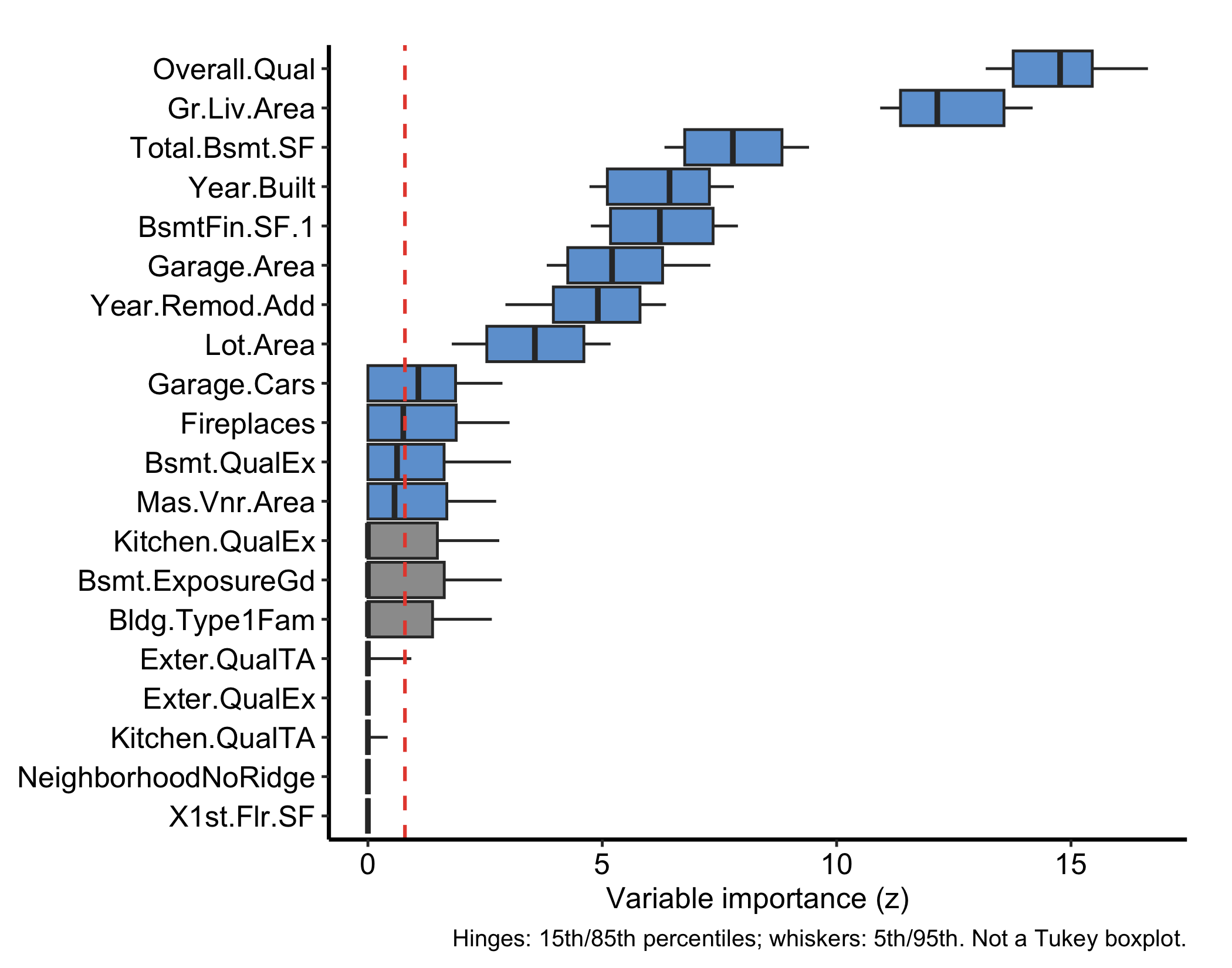
Permutation importance (the VIMP chapter) answers “how much does the forest lean on this variable?” by breaking the variable and watching error rise. varPro (Lu et al. 2026) asks a different question: “how much do the forest’s own splitting rules depend on this variable?” Rather than permuting predictors, it scores each one by how much a tree’s release rules rely on it, and calls the result variable priority. Reach for it when you want a selection that comes with a built-in cutoff (so the method tells you which variables to keep, not just how to rank them), when you want the direction and magnitude of a local effect, or when you want to flag unusual observations the same forest can isolate.

ggRandomForests (Ehrlinger 2026) provides a family of gg_* extractors that pull these scores out of a fitted varpro object and render them as tidy ggplot2 graphics. This chapter works through the main extractors on a regression fit and a classification fit. As elsewhere, each plot() hands back a bare ggplot you finish with a house theme.

29.2 The data it needs

The extractors read from a fitted varpro object, so the input is whatever varpro() itself needs: a formula and a data frame. The outcome type decides the family, and that matters here because several of the extractors are family-specific. We start with a regression fit on the housing data shipped with randomForestSRC (Ishwaran and Kogalur 2026) — 2,930 homes and 80 predictors, modelling sale price (SalePrice). This is the same kind of dataset the random-forest chapters use, and the extra width is the point: variable priority earns its keep when there are far more candidates than you can eyeball.

set.seed(42)
data(housing, package = "randomForestSRC")
o <- varpro(SalePrice ~ ., data = housing, ntree = 100)
plot(gg_varpro(o, nvar = 20)) + theme_hv_manuscript()

Figure 29.1: Variable priority for the top 20 predictors of the housing regression fit, with the dashed cutoff line separating selected from unselected variables

gg_varpro() returns an honest 15/85 boxplot for each variable. With 80 predictors we pass nvar = 20 to show the top-ranked; the box spans the importance values obtained when the variable is released across the rule ensemble, and the dashed reference line at the cutoff (default 0.79 of the top score on the local-standardized scale) separates selected from unselected variables. Variables whose boxes sit to the right of the cutoff are retained.

29.3 Build it

The plot in Figure 29.1 is the core figure. Two variants make it more informative. Setting faithful = TRUE shows the per-tree importance draws as jittered points behind the boxplot, exposing the spread that the summary hides:

plot(gg_varpro(o, faithful = TRUE, nvar = 20)) + theme_hv_manuscript()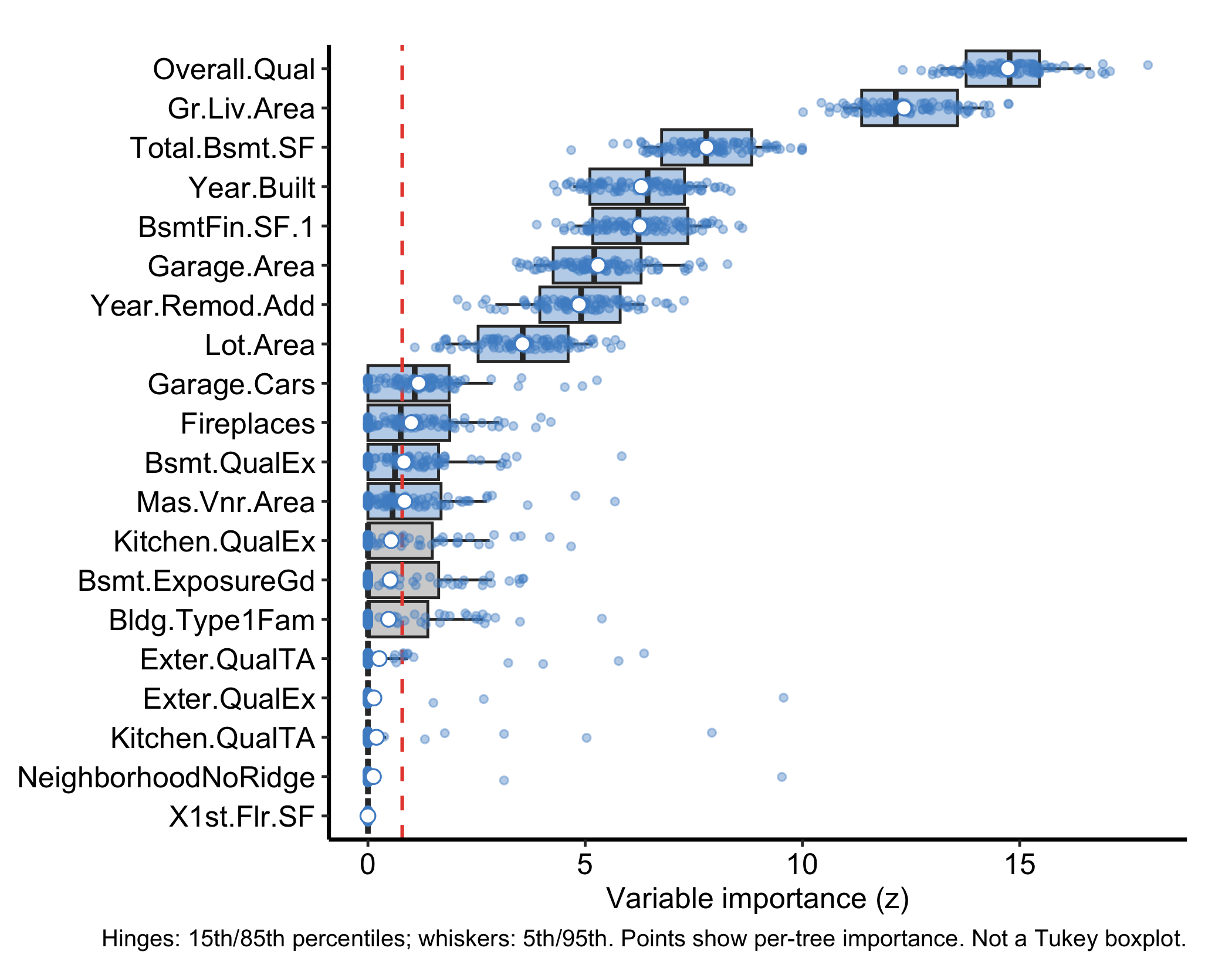

Figure 29.2: The same priority boxplots with per-tree importance draws shown as jittered points behind each box, exposing the spread the summary hides

Setting nvar lower restricts the display further, handy when a wide problem like this one would otherwise crowd the panel and you only want the leaders:

plot(gg_varpro(o, nvar = 8)) + theme_hv_manuscript()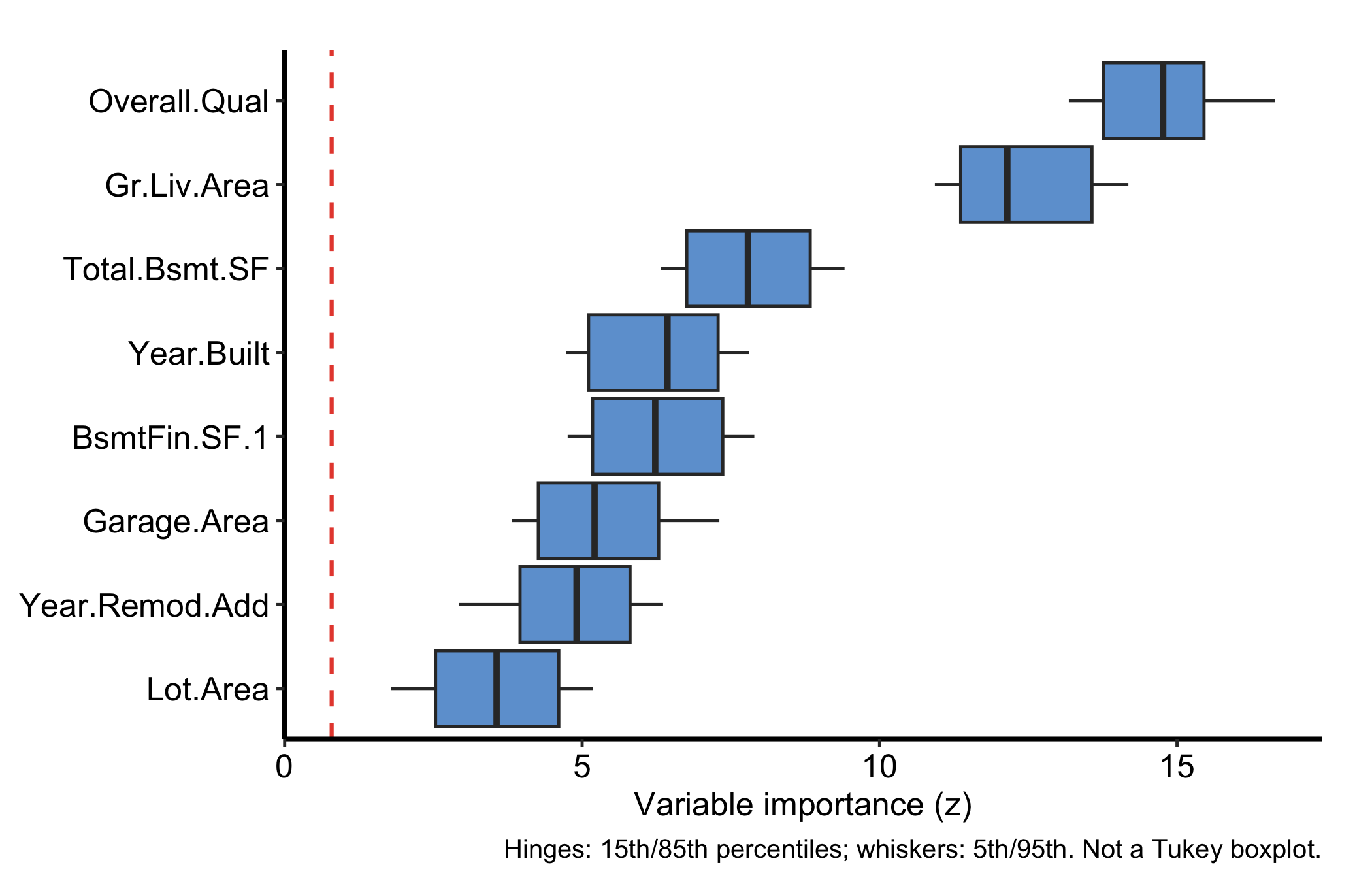

Figure 29.3: Variable priority restricted to the top eight predictors, the leaders-only view for a crowded wide problem

29.4 Read it

The 15/85 boxplot is the figure to learn to read, and the cutoff line is what makes it a selection rather than just a ranking.

The cutoff line decides membership. Boxes to the right of the dashed line are the variables varPro keeps; boxes to the left are set aside. Unlike a VIMP bar chart, where you eyeball the break yourself, the method draws the line for you. You can move it with the cutoff argument when you want to be stricter or looser.
Box width is stability. A tight box means the variable scored consistently across the rule ensemble; a wide box straddling the cutoff is a variable whose selection you should not bet the paper on. Turn on faithful = TRUE to see the raw draws behind the summary.
Priority is not the same as importance. A variable can carry high priority (the rules depend on it) without the large error jump that permutation VIMP rewards, and vice versa. Read the two methods as complementary views, not as two attempts at the same number.

29.5 Variations

29.5.1 Beta-refined importance (regression only)

gg_beta_varpro() is regression-only. Within each release region it fits a lasso and reports the refined slope (β) coefficients instead of a VIMP-style importance, so you get not just whether a variable matters but the direction and magnitude of its local linear effect.

plot(gg_beta_varpro(o)) + theme_hv_manuscript()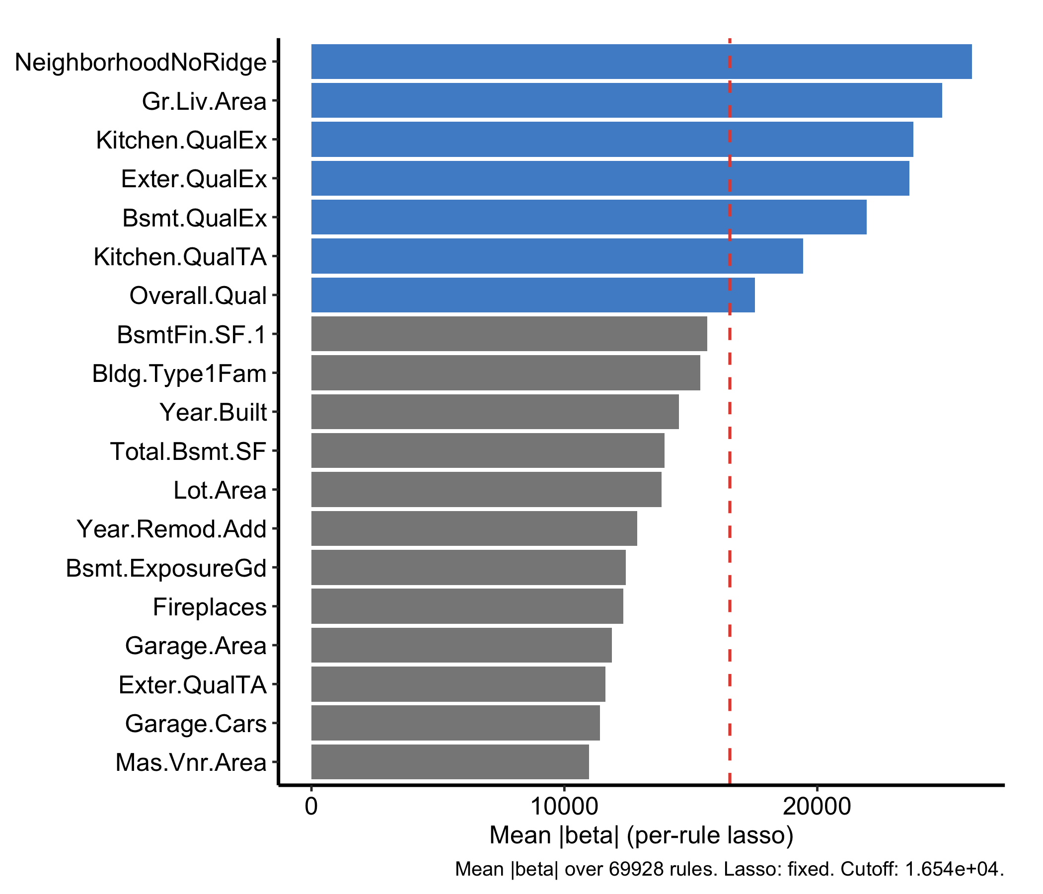

Figure 29.4: Beta-refined importance for the housing regression fit, reporting lasso slope coefficients that carry direction and magnitude rather than VIMP-style scores

The per-rule lasso refinement (beta.varpro) is the expensive step; under Quarto’s freeze the result is cached after the first render. Because these are lasso-refined β coefficients rather than importance scores, they can be negative.

29.5.2 Individual variable priority

gg_ivarpro() computes individual (observation-level) variable priority, decomposing the forest importance down to each case. On a regression fit with weak per-observation signal the decomposition can collapse to nothing (it returns zero rows), so we demonstrate it on a classification forest, which also lets us show the which_class argument. We fit status ~ . on the breast data (also from randomForestSRC): 198 patients, 32 predictors, and a two-level recurrence outcome (N = no recurrence, R = recurrence).

set.seed(42)
data(breast, package = "randomForestSRC")
oc <- varpro(status ~ ., data = breast, ntree = 100)
plot(gg_ivarpro(oc)) + theme_hv_manuscript()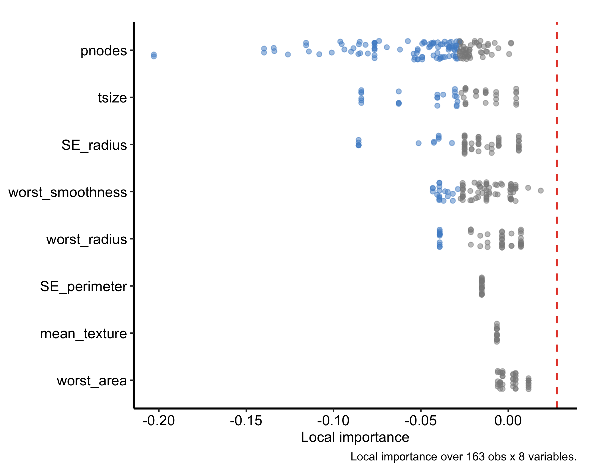

Figure 29.5: Individual variable priority for the breast classification fit, decomposing forest importance down to each observation

Each panel summarises how strongly individual observations rely on a given variable. You can focus on a single outcome level with which_class — here the recurrence class:

plot(gg_ivarpro(oc, which_class = "R")) + theme_hv_manuscript()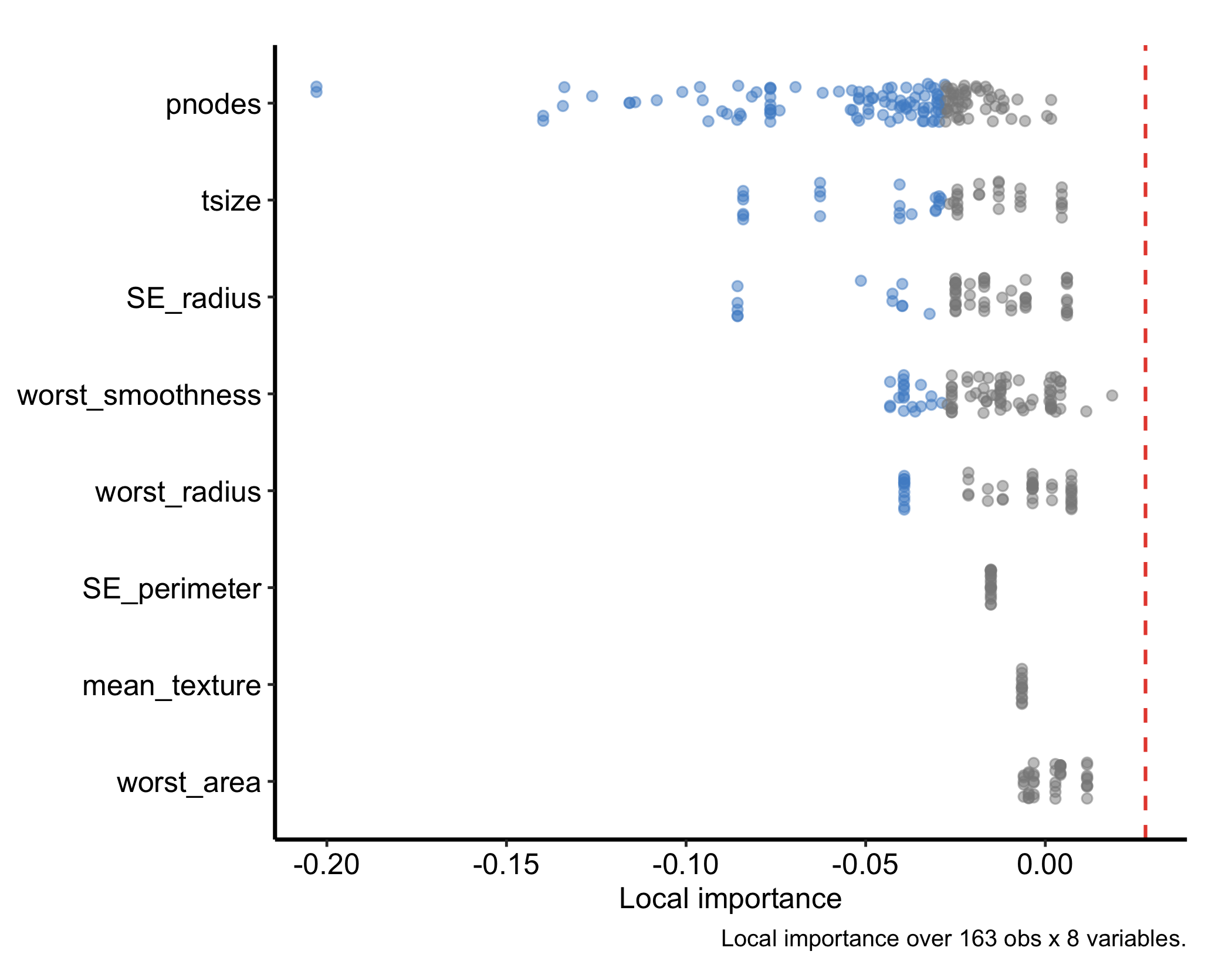

Figure 29.6: Individual variable priority focused on the recurrence class of the breast fit via the which_class argument

29.5.3 Conditional priority by class

The classification fit also supports conditional = TRUE in gg_varpro(), which facets the priority bars by outcome class so you can read which predictors separate which classes. This option needs a classification forest; it errors on the regression fit.

plot(gg_varpro(oc, conditional = TRUE, nvar = 15)) + theme_hv_manuscript()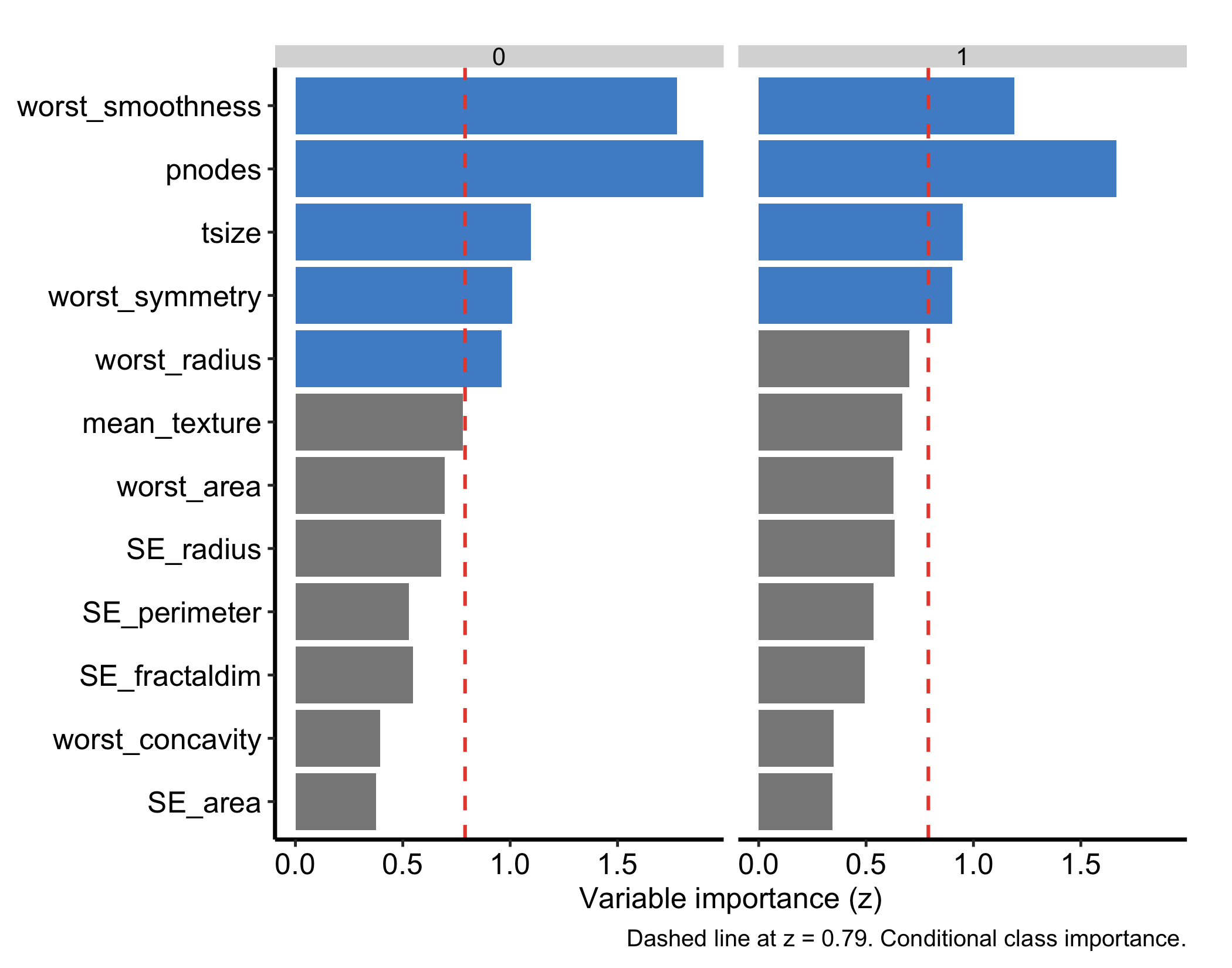

Figure 29.7: Conditional variable priority faceted by outcome class, showing which predictors separate which classes in the breast fit

29.5.4 Anomaly / isolation scores

gg_isopro() visualises in-sample anomaly (isolation) scores. These come from an isopro object, and there is no .varpro method that builds one for you: you construct it first with varPro::isopro() on the fitted forest, then pass that to gg_isopro().

iso <- isopro(object = o, ntree = 100)
plot(gg_isopro(iso)) + theme_hv_manuscript()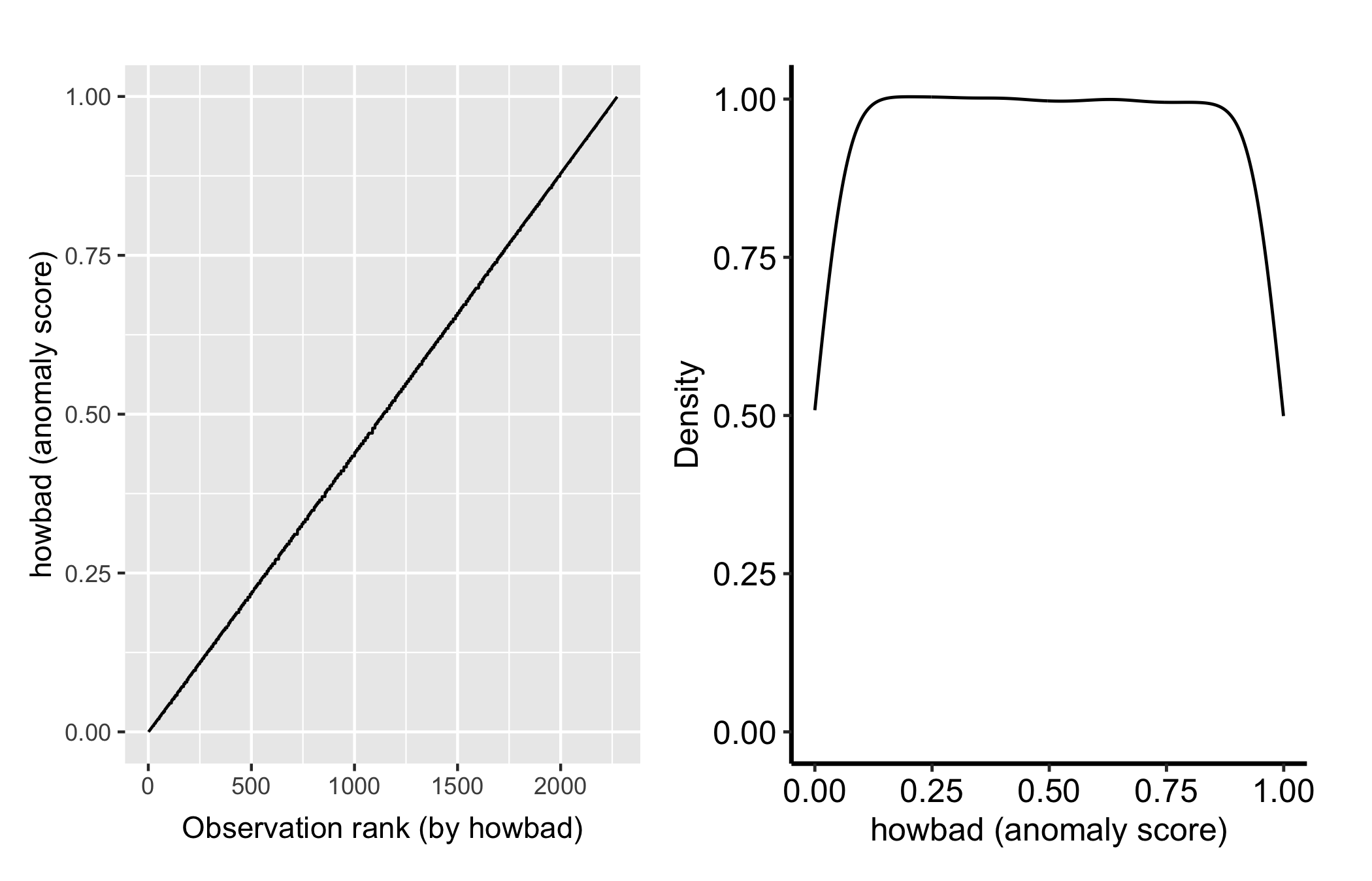

Figure 29.8: In-sample anomaly scores from an isolation forest, where higher scores flag observations the forest separates with few splits

Higher isolation scores flag observations the forest separates with few splits, candidate outliers. Pass newdata to gg_isopro() to score held-out observations against the fitted isolation forest.

29.5.5 Partial dependence

The extractors so far rank and refine variables; partial dependence asks how a selected variable moves the prediction. gg_partial_varpro() runs varPro::partialpro() on the fitted forest and draws a marginal-effect curve per variable, with a scale argument that sets the y-axis to suit the outcome family. Because that treatment spans regression, classification, and survival, it gets its own chapter — see varPro partial dependence. (gg_partialpro() is the superseded name for this extractor; it is now a thin alias for gg_partial_varpro(), so reach for the new name.)

29.6 Unsupervised variable dependence

Everything above needs an outcome. varPro::uvarpro() drops that requirement: it fits an unsupervised forest and scores how strongly each variable depends on the others, with no response to predict. gg_udependent() reads those cross-variable scores and draws them as a dependency graph — nodes are variables, edges the dependencies between them — so you can see which predictors travel together before any modelling. Reach for it when you want to understand the structure among the predictors themselves, for example to spot a cluster of collinear measurements.

set.seed(42)
num_cols <- names(housing)[vapply(housing, is.numeric, logical(1))]
uv <- uvarpro(housing[, setdiff(num_cols, "SalePrice")], ntree = 100)
plot(gg_udependent(uv)) + theme_hv_manuscript()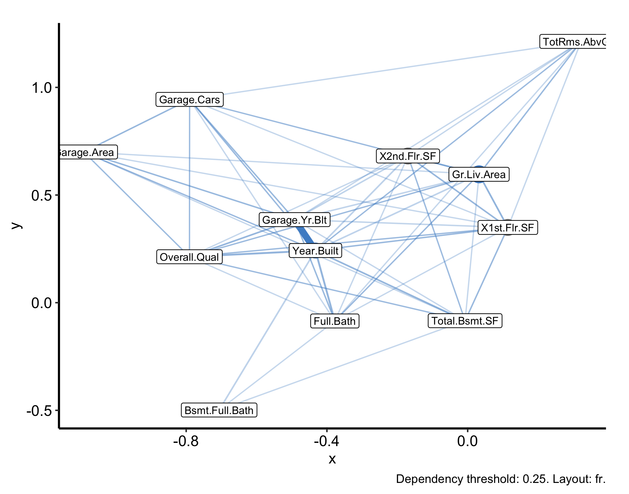

Figure 29.9: Unsupervised dependency graph among the numeric housing predictors, where thick edges mark strongly interdependent variables

We fit it on the numeric housing predictors (with the SalePrice outcome and the factor columns dropped — the dependency graph is built from a numeric distance and cannot square a mixed-type design). A thick edge between two variables means the forest finds them strongly interdependent; an isolated node is a variable that carries information the others do not.

29.7 Pitfalls

gg_isopro() needs an isopro object first. There is no .varpro method, so calling gg_isopro() on the varpro object directly fails. Build iso <- isopro(object = o, ...) and then plot iso.
gg_beta_varpro() is regression-only. The lasso β refinement is defined for a regression fit; do not expect it off a classification varpro object.
conditional = TRUE needs a classification forest. gg_varpro(conditional = TRUE) facets priority by class, so it errors on a regression fit like the housing model. Use it on a classification fit such as the breast one.
gg_ivarpro() needs real signal. Individual priority decomposes importance to each observation, and on a weak problem that decomposition can return zero rows and an empty plot. It works on a strong-signal fit like the breast classification forest, which is why the individual-priority examples use it.
gg_udependent() needs all-numeric data. The unsupervised dependency graph is built from a numeric distance, so a mixed-type design (factors plus numerics, like the full housing frame) fails with “Adjacency matrices must be square.” Pass only the numeric columns, as the example does.
Wide data needs nvar/nvars. With 80 predictors the bare gg_varpro() and gg_partial_varpro() displays are unreadable walls; cap them with nvar (the boxplot) and nvars (which variables partialpro even computes, the expensive step).