A random forest is an ensemble: its prediction is an average over many trees. That raises the first practical question of every fit, before you read a single importance ranking or survival curve. How many trees are enough? Too few and the average is still jittering from tree to tree; the rankings and curves you draw from it will shift if you refit. Enough, and the forest has settled into a stable prediction you can build on.
Reach for gg_error() whenever you have just fit a forest and want to confirm it converged. It reads the OOB (out-of-bag) error the forest recorded as it grew and plots that error against the number of trees. Each observation is predicted only by the trees that did not see it during training, so the OOB error is an honest, cross-validation-like estimate computed for free while the forest grows. The curve it produces is the single cheapest diagnostic in the random-forest workflow, and it is the one to look at first.
24.2 The data it needs
gg_error() does not work on a data frame. It works on a fitted rfsrc object, and it needs that object to have recorded its error history. By default rfsrc() records the OOB error only at the final tree, which leaves a single number and nothing to plot. The fix is one argument at fit time: block.size = 1 tells the forest to record the OOB error after every tree.
We use the veteran survival data again, one row per patient with a follow-up time and an event status, and grow 100 trees.
                         Sample size: 137
                    Number of deaths: 128
                     Number of trees: 100
           Forest terminal node size: 15
       Average no. of terminal nodes: 5.96
No. of variables tried at each split: 3
              Total no. of variables: 6
       Resampling used to grow trees: swor
    Resample size used to grow trees: 87
                            Analysis: RSF
                              Family: surv
                      Splitting rule: logrank *random*
       Number of random split points: 10
                          (OOB) CRPS: 62.83683172
             (OOB) standardized CRPS: 0.06289973
   (OOB) Requested performance error: 0.30737632
The printed summary confirms the family (survival), the number of trees, and the error rate at the final tree. gg_error()(Ehrlinger 2026) turns that final number into the whole history.
24.3 Build it
With the forest fit and block.size = 1 in place, the plot is one line. gg_error() pulls the cumulative OOB error after each additional tree. For a survival forest the error is 1 - C-index (the concordance index, the probability the model ranks a random pair of patients in the right order), so lower is better.
plot(gg_error(rf)) +theme_hv_manuscript()
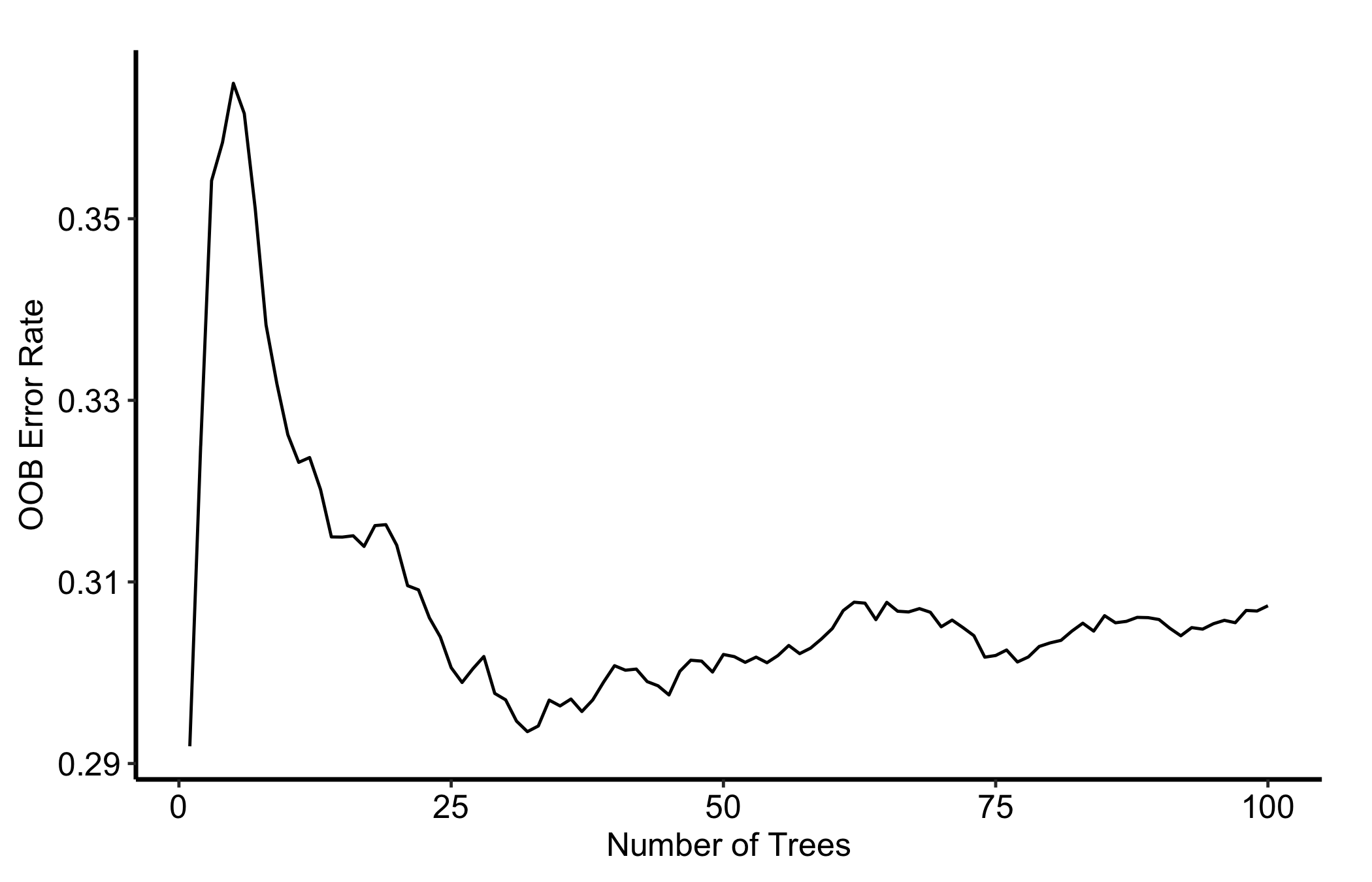
Figure 24.1: Out-of-bag error against the number of trees for a 100-tree survival forest, flattening well before the final tree
The result plots error on the y-axis against the number of trees on the x-axis. rfsrc()(Ishwaran and Kogalur 2026) did the work; gg_error() just reads it back.
24.4 Read it
A convergence curve tells its story by its shape, not its level. Three things to look at:
The drop on the left. While the first few dozen trees are added, each new tree still carries information the ensemble did not already have, so the error falls quickly.
The flat tail on the right. A tail that has gone flat means additional trees no longer change the prediction. The forest has converged, and you have grown enough trees.
A tail still sloping down. If the curve is still trending downward at the right edge, the forest is not done improving. That is your signal to refit with a larger ntree.
Here the curve is essentially flat well before 100 trees, so for this small dataset 100 trees is adequate. Make this glance a habit: check gg_error() before you trust any downstream importance or dependence plot, because those are only as stable as the forest underneath them.
24.5 Variations
24.5.1 A forest that has not converged
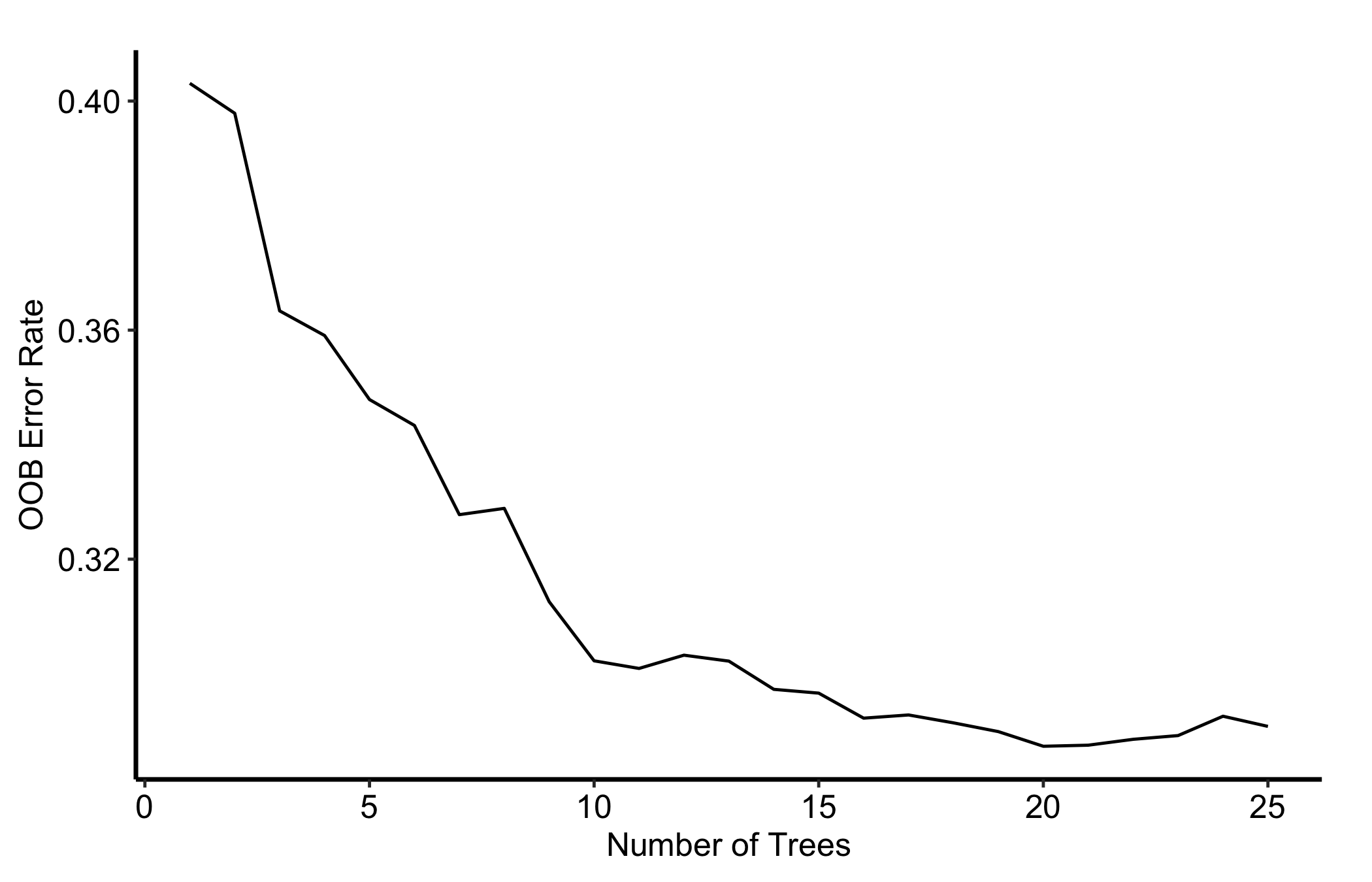
To see what an undersized forest looks like, refit with far too few trees. The curve never reaches a flat tail; it is still descending at the right edge, which is precisely the pattern that should send you back to a larger ntree.
Figure 24.2: Out-of-bag error for an undersized 25-tree forest, still descending at the right edge instead of flattening
Compare this to the 100-tree curve in Figure 24.1. The shape, not the number on the axis, is what tells you whether to grow more trees.
24.6 Pitfalls
Forgetting block.size = 1. This is the one that bites everyone. Without it, rfsrc() records OOB error only at the final tree, so gg_error() has a single value and the convergence curve collapses to one point. Set it at fit time whenever you intend to inspect convergence.
Reading the level instead of the shape. The y-axis value depends on the outcome and the cohort; a 1 - C-index of 0.4 is not “bad” in any absolute sense. What you are reading is whether the curve has flattened, not where it sits.
Mistaking OOB error for an external test. The OOB estimate is honest and free, and it is the right tool for judging convergence. It is not a substitute for an external validation set when the cohort is small: with few patients the OOB error itself is noisy, and a flat curve confirms the forest settled, not that it will generalize to a new institution.
Ishwaran, Hemant, and Udaya B. Kogalur. 2026. randomForestSRC: Fast Unified Random Forests for Survival, Regression, and Classification (RF-SRC). https://www.randomforestsrc.org/.